||||
|\/|
|/\|
||||
David L. Duffy, MBBS PhD.
Queensland Institute of Medical Research,
300 Herston Road,
Herston, Queensland 4029, Australia.
Email: davidD@qimr.edu.au
Last Updated: 2012-09-11
Sib-pair is a computer program for the manipulation and statistical analysis of genetic datasets. It implements a simple interpreted language in which the user writes commands. These can be entered interactively, or submitted as a batch from a text file in the usual way.
I have developed the program over a number of years in the open software way of "scratching an itch". That is, Sib-pair carries out practical procedures which I have required in the day-to-day handling of genetic data, and were not available using other computer programs and/or were interesting as a research or educational question.
These include:
There are also a variety of standard statistical procedures, such as multiple regression analysis (including unconditional and conditional logistic regression), principal components analysis, contingency table analysis, survival analysis, random number generators, quantiles for assorted statistical distributions.
Finally, there are a few utilities that give expectations for specified genetic models eg recurrence risks for a single major locus model, and can carry out file manipulations.
In this document, I try to give a gentle introduction to using Sib-pair. The other sources of information about Sib-pair are the manual, the extended help pages for each command, and reading the Fortran 95 source code (it does have some comments!).
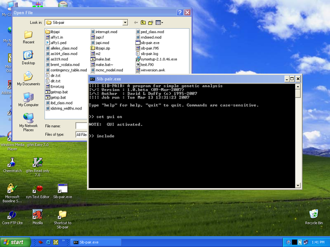
Sib-pair is not difficult to use. In a Windows environment, double-click the icon or open a DOS box in your working directory (folder) and call Sib-pair from the command line. The latter assures that Sib-pair will find your pedigree files and write output in the same directory. In a Unix environment, run Sib-pair from the command line.
davidD@moonboom:~$ sib-pair |||| SIB-PAIR: A program for simple genetic analysis |\/| Version : Version 1.00.beta g95 (17-Aug-2012) |/\| Author : David L Duffy (c) 1995-2012 |||| Job run : Tue Sep 11 12:15:00 2012 (orpheus.qimr.edu.au) Type "help" for help, "quit" to quit, "ctrl-C" to interrupt. >> |
You see much the same on Windows.
|
|
Now type in "help" on the command line (followed by <ENTER>):
>> help Keywords can be shortened to the first 3 letters. Help prints a brief description of a command or group of commands: help [ <search string> | All | Globals | Operators | Data | Analysis | Examples] For full online help: $ your_favourite_HTML_browser sib-pair.html Now try "help Examples" |
Entering "help All" gives a long list of all the commands (see Appendix).
To list just the commands mentioning "merlin":
>> help merlin
rea loc mer <fil> {read Merlin locus file}
wri mer [dum] <fil> {write Merlin pedigree file}
wri loc mer <fil> {write Merlin locus file}
wri map mer <fil> {write Merlin map file}
|
The latter three commands can produce the files needed to run a multipoint linkage analysis in MERLIN.
Here is the list of commands mentioning "risk". Then we will try the "sml" (short for single major locus) command.
>> help risk
sml <pA> <penAA> <penAB> <penBB> {recurrence risks}
grr <prev> <pA> <GRR> [<add|dom|rec>] {recurrence risks}
hrr <tra> [<c_op> <thr>] {haplotype relative risk}

>> sml 0.17 0.21 0.08 0.03

------------------------------------------------
Single Major Locus Recurrence Risk Calculation
------------------------------------------------

 Frequency(A): 0.170000; Pen(AA): 0.210; Pen(AB): 0.080; Pen(BB): 0.030
 Trait Prev  : 0.049312; Pop AR:  39.2%; Var(Add): 0.001141; Var(Dom): 0.000127

 Measure      MZ Twin       Sib-Sib        Par-Off      Second
----------   ----------    ----------     ---------    ----------
 Rec Risk         0.075         0.062         0.061         0.055
 Rel Risk         1.564         1.264         1.250         1.124
 Odds Rat         1.610         1.281         1.266         1.131
 PRR              1.522         1.248         1.235         1.117
 Tet Corr         0.106         0.054         0.051         0.026
 ibd|A-A          1.000         0.552         0.500         0.276
 ibd|A-U          1.000         0.497         0.500         0.248

 Freq of A if Affected: 0.351983 (0.123,0.458,0.419)
 Freq of A if Unaffctd: 0.160561 (0.024,0.273,0.703)

 Mating       Proportion    Risk to offspring
----------   -----------   ------------------
UnA x UnA         0.904         0.048
Aff x UnA         0.094         0.060
Aff x Aff         0.002         0.075
|
The "sml" results show that a gene with the given allele frequency and penetrances (APOE*E4 and Alzheimer's disease by age 75) give rise to a recurrence risk of 6.2% in siblings of cases, a 1.3-fold increase in risk compared to the baseline population risk of 4.9%. The frequency of the risk allele (here APOE*4) is doubled in cases when compared to controls, and IBD sharing (Identity-by-Descent) in affected sib pairs is expected to be 55%.
Simultaneously pressing the combination of the "Ctrl" and "c" keys interrupts whatever calculation Sib-pair is currently doing and returns you back to the Sib-pair command prompt. Usually Sib-pair will first try to complete a part of the calculation and give a result, so there may be a small delay. Pressing "Ctrl-C" multiple times causes the Sib-pair to stop completely, and returns you to the operating system.
Two last things:
>> 1+1 ; 2+2 => 2. => 4. >> quit This job took 28.1 minutes |
In this case, I will go through the analysis of some pedigree data from beginning to end. I won't describe the commands in too much detail, as they will be covered later.
Usually, I have:
Here is a diagram of a pedigree described in a paper by Lawler and Sandler (1954) where members are affected by the condition familial elliptocytosis.
The diagram in Morton (1956):

And here is the same diagram amended to include some additional necessary family members, and recoding the alleles to 1, 2, and 3 (Sib-pair only allows single letter or numerical allele codes):
                               [101]   (102)
                                 |       |
                                 +---+---+
                                     |
              +----------------------+-----------------------------------------------+
              |                                                                      |
      [201] (202)                                                            (203) [204]
        |     |                                                                |     |
        +--+--+                                                                +--+--+
           |                                                                      |
  +--------+--+------------+-----------+----------------------+             +-----+-----+
  |           |            |           |                      |             |     |     |
(301) [302] (303)  [304] [305]       (306) [307]      [308] (309) [311]   (310) (312) [314]
 Aff   UnA   Aff     ?    UnA         Aff   UnA         ?    Aff   UnA     Aff   UnA   Aff
 1 3   x x   1 3    x x   3 3         1 3   x x        x x   1 3   x x     1 2   2 3   3 3
  |     |     |      |                 |     |          |     |     |       |
  +--+--+     +--+---+                 +--+--+          +----++     +------++
     |           |                        |                  |             |
     |     +-----+-----+-----+           ++----+-----+     +-+-------+     |
     |     |     |     |     |           |     |     |     |         |     |
   [405] [407] [408] [409  [410] [412] (411) [413] (414) [415](417)(418) (419)
    UnA   UnA   Aff   Aff   Aff    ?    Aff   Aff   UnA   Aff   ?   Aff   UnA
    3 3   2 3   1 1   1 2   1 1   x x   1 1   1 3   3 3   1 3  x x  1 3   2 2
                              |    |                            |    |
                              +--+-+                            +--+-+
                                 |                                 |
                                 |                           +-----+-----+
                                 |                           |     |     |
                               (504)                       [505] [506] (507)
                                Aff                         Aff   Aff   Aff
                                1 3                         1 1   1 1   1 1
Note every pedigree member has been given a unique identifier. In the later generations, there is information as to whether individuals are affected or unaffected (by elliptocytosis), and their genotype at the Rhesus blood group locus. Each genotype is given as the two alleles.
From this, I will make a single plain text file that contains all this information in the form that Sib-pair reads. The pedigree is written as one line per pedigree member. Each line contains the same number of items separated by spaces. The columns are:
| Column | Name |
|---|---|
| 1 | Pedigree name |
| 2 | Individual identifier |
| 3 | Father's identifier |
| 4 | Mother's identifier |
| 5 | Sex (m or f) |
| 6 | Affected or unaffected by elliptocytosis (y or n) |
| 7 | First allele of Rhesus genotype (1, 2 or 3) |
| 8 | Second allele of Rhesus genotype (1, 2 or 3) |
Because columns are "free format" white-space separated, if a value is missing, there must be a placeholder to identify the column (Sib-pair uses an "x" for this purpose).
I use the gvim text editor, but you can use NotePad or any other editor. We open a new document. Now we go through the pedigree diagram person by person, adding one line to our document for each person. The first record (for person 101) will be:
ped5 101 x x m x x x
The parent identifiers are set to "x" because they are not given. Furthermore the trait status and genotype are also unknown. Where sex is not given in the diagram, we will assign them so that the marriages in the drawing are consistent.
The first "nonfounder" (that is a person with parents included in the diagram) is written as:
ped5 202 101 102 f x x x
Skipping forward, the last pedigree record will be:
ped5 507 417 418 f y 1 1
The pedigree columns now need to be identified in such a fashion that Sib-pair can recognize them. At the start of the file, I first prepend a comment, so I know what this file does. Comment lines are ignored by Sib-pair and are prefixed by a "#" at the start of the line:
#
# Elliptocytosis pedigree 5 from Lawler & Sandler 1954, Morton 1956
# Zmax of 3.31 at c=0.05
#
Following this, we declare the columns. The first five columns are standard and so don't need to be named. The sixth column is disease state, so the first line of the declarations (using the "set locus" command) is:
set locus ellipto affection
The seventh and eight columns represent the alleles of the genotype, so the second declaration line is:
set locus rhesus marker
To show where the pedigree data starts, we add a line:
read pedigree inline
The end of the pedigree data is marked by ";;;;" on its own line. After this we add the "run" command, which tells Sib-pair to process the pedigree. We save the completed script to a file "ellipto5ex.in". Its contents looks like this.
So we can start up Sib-pair, and "include" the contents of this file into our session:
>> include ellipto5ex.in |
If you got the message
>> include ellipto5ex.in ERROR: Unable to open "ellipto5ex.in". |
Then you are not in the correct directory (folder). The "pwd" command in Sib-pair shows you which directory you are in, and can be used to change directory as well. Alternatively, you can try again, using just
>> include |
which will give you some type of file chooser menu. This will allow you to navigate to the correct directory and include the file. You should now get:
Reading commands from "ellipto5ex.in". ! ! Elliptocytosis pedigree 5 from Lawler & Sandler 1954, Morton 1956 ! Zmax of 3.31 at c=0.05 ! Pedigree file = inline.ped Number of loci = 2 Locus Type Position --------------- ---- ---------------- ellipto a 6 rhesus m 7-- 8 Number of marker loci= 1 Bonferroni corr. 5% = 0.050000 Bonferroni corr. 1% = 0.010000 Bonferroni corr. 0.1%= 0.001000 Max record length is 25 characters Screened 1 pedigrees, 36 records (0.00 s). Read in 1 pedigrees, 36 individuals (0.01 s). Dataset occupies 0.002 Mb. No sex-informative markers. Nuclear family error checking. Nuclear family error checking completed. Number of data problems = 0 Starting values for missing genotypes generated. |
Total number of pedigrees = 1 Number with only 1 member = 0 Total number of sibships = 10 Total number of subjects = 36 Total subjects genotyped = 23 (63.9%) Total number of genotypes = 23 Largest pedigree (members) = 36 Mean size of pedigrees = 36.0 Closing include file "ellipto5ex.in". >> |
So I have successfully read in the pedigree data, and there are no messages about errors of various types. The "describe" command tells me about the phenotype (ellipto) and genotypes (rhesus):
>> describe

------------------------------------------------
Segregation ratios for trait "ellipto   "
------------------------------------------------

Total sample   All       Fndrs     Nonfndrs
-------------------------------------------
   Aff/Tot    17/  23    0/   0   17/  23
   Prop Aff     0.739     0.000     0.739
   Missing         13        11         2

Mating Type     UxU       UxA       AxA
-------------------------------------------
   Matings          0         0         0
   Aff/Tot     0/   0    0/   0    0/   0
   Prop Aff     0.000     0.000     0.000

Relative pair   RecRisk     Aff-Aff     Aff-UnA  Tetrachoric r
-----------------------------------------------  -------------
   Marital        0.000           0           0        0.000
   Gparent        1.000           4           0        1.000
   Halfsib        0.000           0           0        0.000
   Par-Off        0.846          11           4        0.629
   Fullsib        0.732          15          11        0.000
   MZ twin        0.000           0           0        0.000

------------------------------------------------
Allele frequencies for locus "rhesus"
------------------------------------------------
   Allele  Frequency   Count  Histogram
       1     0.4783       22  **********
       2     0.1304        6  ***
       3     0.3913       18  ********

Number of alleles    =    3
Heterozygosity (Hu)  =    0.6145
Poly. Inf. Content   =    0.5181
4 Neff mu (SSMM)     =    2.44529900
Number persons typed =     23 ( 63.9%)
|
I can see that 17 pedigree members are affected by the condition, and that there are 23 individuals genotyped. The "hwe" command doesn't suggest marker problems.
>> hwe -------------------------------------------------- Hardy-Weinberg equilibrium for marker loci -------------------------------------------------- Marker Typed Genos Chi-square Asy P Emp P Iters -------------- ------ ------ ---------- ------ ------ ------ rhesus 23 6 1.2 0.7496 0.8696 23 HWE . |
Is there genetic linkage between familial elliptocytosis and Rhesus blood group? Sib-pair offers a nonparametric identity-by-descent test of linkage ("apm"):
>> apm ellipto ibd

------------------------------------------------
APM for trait "   ellipto" v. all markers
------------------------------------------------

NOTE:  Identity-by-descent based statistic used.


Marker         NFams  NAff   Z-value    Asy P  Emp P  Iters
-------------- ------ ------ ---------- ------ ------ ------
    rhesus          1     17        1.7 0.0443 0.0700    200 APM-IBD +
    rhesus          1     17        4.1 0.0000 0.0050    200 GPM-IBD ***
|
There are results from two tests here, one using affected pedigree members only (APM), and the other including information from unaffecteds as well (GPM). The latter is more impressive, with a Z-score of 4.1 being the equivalent of a lod score of
>> 4.1^2 / (2*log(10)) => 3.650245120396831 |
This score seems a bit high perhaps (I know that the parametric lod score is only 3.3). Like many Sib-pair tests, this test is simulation based, so it is worthwhile increasing the number of simulations used to refine the estimates:
>> set iterations 10000
>> apm ellipto ibd

------------------------------------------------
APM for trait "   ellipto" v. all markers
------------------------------------------------

NOTE:  Identity-by-descent based statistic used.

Marker         NFams  NAff   Z-value    Asy P  Emp P  Iters
-------------- ------ ------ ---------- ------ ------ ------
    rhesus          1     17        1.4 0.0757 0.0852  10000 APM-IBD +
    rhesus          1     17        4.3 0.0000 0.0024  10000 GPM-IBD ***
|
So, elliptocytosis seems to be linked to this marker, but the empirical P-value is equivalent to a lod of 2. We can look at some other linkage tests, including the original Penrose sib-pair linkage test:
>> pen ellipto rhesus

---------------------------------------------------------------
Penrose Sib Pair Linkage Analysis for "ellipto" v. "rhesus"
---------------------------------------------------------------

                     rhesus
ellipto    Concordant  Discordant
Concordant         11           4
Discordant          0          11

No. of sib pairs   =    26
No. of sibships    =     6

    No. complete observations =    26
    LR contingency chi-square =  18.03
           Degrees of freedom =   1
           Asymptotic P-value =   0.0000
              Empiric P-value =   0.0001 ( 2600000 MCMC iterations)
             Trend chi-square =  13.44   (P=0.0002)
                    Agreement =   0.846  (   22/   26)
                Cohen's Kappa =   0.6994
|
We can also look at this using the assoc test:
>> set plevel 1
>> assoc ellipto

--------------------------------------------------
Allelic association testing for trait "ellipto"
--------------------------------------------------

  ---- Association Analysis for "rhesus    "------
    Allele  Affected    Unaffected    Total    Dev
  ------------------------------------------------
     1       22 (.647)      0 (.000)      22    8.1
     2        2 (.059)      4 (.333)       6    0.4
     3       10 (.294)      8 (.667)      18    2.9
  ------------------------------------------------
   Total     34            12             23

       No. trait(+) marker(-) =     0
       No. trait(+) marker(+) =    23
                Fis, Fit, Fst =   0.0818   0.4125   0.3602
   Contingency Pearson chi-sq =  16.0
   Nominal degrees of freedom =   2
              Nominal P-value =   0.0003
      Equalled or exceeded by =   1/10001 simulated values (0.0001)
 Mean (Var) simulated chi-sqs =   1.7 (   2.7)

 -------- Combined transmission test for "    rhesus" --------
   Allele   Affected   Unaffected   Total   E(Aff)    Z    P
 -------------------------------------------------------------
     1       13 (.59)      0 (.00)     13    7.9    2.8 0.0053
     2        2 (.09)      2 (.25)      4    2.4   -0.4 0.6653
     3        7 (.32)      6 (.75)     13   11.7   -2.6 0.0094
 -------------------------------------------------------------
   Total     22            8           30

                    marker(-) =     1
       No. trait(+) marker(+) =    15
          No. useful sibships =     4
 Global association statistic =   2.5
           Degrees of freedom =   2
      Equalled or exceeded by =  20/ 1019 simulated values (0.0196)
 Mean (Var) simulated chi-sqs =   0.5 (   0.3)
|
Because the assoc empirical P-value is generated by gene dropping, in a single pedigree like this it gives a valid test of cosegregation of alleles at the Rhesus locus with elliptocytosis. The "1" allele was never seen in an unaffected individual. The FBAT (combined transmission test) confirms children with elliptocytosis received the "1" allele more often than expected.
Now I'll use Sib-pair to output the files that Superlink requires for a parametric linkage analysis. I'll model elliptocytosis as due to a rare fully penetrant dominant locus:
>> set sml 0.0001 1 1 0 SML model: P(A)=0.000100 Pen(AA)=1.000 Pen(AB)=1.000 Pen(BB)=0.000 >> write locus linkage el.loc Writing LINKAGE type locus file: el.loc >> write ppd el.ppd Writing post-Makeped Linkage style pedigree file: el.ppd |
I'll then change a couple of parameters (the starting recombination distance between ellipto and rhesus, and the evaluation step size) in the locus file "el.loc" using my favourite text editor. Then I'll run Superlink (for this to work you must have already installed Superlink into your directory path):
>> $ gvim el.loc
>> $ superlink el.loc el.ppd

....
                -6.391669        -51.787565     3.265655
                -5.268026        -51.752765     3.280768
                -4.169080        -51.760457     3.277427
                -3.093770        -51.834167     3.245415
                -2.041100        -52.026618     3.161835
                -1.010135        -52.505211     2.953985
   rhesus
                0.000000         -56.912210     1.040050
--------------------------------------------------------------
  MAX           -5.268026        -51.752765     3.280768
--------------------------------------------------------------
|
The maximum lod is 3.28 at 5.3 cM distant from the marker. The Rh-linked elliptocytosis gene (EPB41) is now known to lie at 29.2 Mbp from the 1p telomere (1p33-p32), and the Rhesus complex of genes at about 25.5 Mbp. They are separated by approximately 3.9 cM on the Rutgers linkage map.
We can actually fit the equivalent model in Sib-pair by creating a marker to represent elliptocytosis. and using the lod command.
>> set locus traitlocus marker
>> if (ellipto) then traitlocus="1/2"
>> if (not ellipto) then traitlocus="1/1"
>> set freq traitlocus 0.9999 0.0001

NOTE:  The marker "traitlocus" has prespecified allele frequencies:
       1=0.9999 2=0.0001

>> lod traitlocus rhesus

------------------------------------
Two-point lod score linkage analysis
------------------------------------

NOTE:  Population allele frequencies for "traitlocus" are prespecified as:
       1=0.9999 2=0.0001

"traitlocus" (2 alleles) v. "rhesus" (3 alleles).

 LogLikelihood   LOD       Theta
--------------  ---------  -------
    -59.3092        0.000   0.5000
    -56.2217        1.341   0.0001
    -52.5057        2.955   0.0100
    -51.9104        3.213   0.0250
    -51.7533        3.282   0.0500
    -51.8939        3.220   0.0750
    -52.1640        3.103   0.1000
    -52.9107        2.779   0.1500
    -53.8264        2.381   0.2000
    -55.9736        1.449   0.3000
    -58.2181        0.474   0.4000

>> quit

This job took   8.8 minutes
|
There are over two hundred different commands in Sib-pair now (see Appendix). The language has an irregular grammar (like all good computer languages), with a mixture of three sorts of statements:
These act upon two types of data:
A scalar constant is either a number or a genotype value. A genotype is made up of two alleles separated by a forward slash and enclosed in a set of double quotes. Each allele can take the values 1...999 or a single letter A...Z and a...z (noting that "x" is reserved as a missing allele).
>> 10 => 10. >> "a/b" => a/b |
There are a few named constants:
>> pi => 3.14159265359 >> y => 1. >> n => 0. >> x => MISS >> . => MISS |
A variable is a column or vector of values in the dataset, and is identified by a unique variable name. The dataset is a rectangular matrix of numbers or genotypes (stored in computer memory), each row representing data for an individual. A variable can be of eight types:
| marker | autosomal genotype |
| xmarker | X-chromosome genotype |
| ymarker | Y genotype |
| mitchondrial | mitochondrial |
| haploid | Y or mitochondrial genotype |
| affection | dichotomous trait value |
| categorical | categorical trait value |
| quantitative | continuous trait value |
The name and column location of a variable is declared by using the set locus command. Usually the values for a variable will be read into Sib-pair from a file (see below). Each row of the dataset is associated with a pedigree and individual ID, IDs of parents of the individual, sex of the individual.
The "head" command prints out the first 10 values of each variable. One can get an equivalent result using the "print" command:
>> head ! ! S p ! e A r ! Per Fat Mot x D onset age D14S52 D14S43 D14S53 o ! AM 101 x x m y 43.0000 x x/x x/x x/x n AM 102 x x f n 77.0000 77.0000 83/87 183/183 151/151 n AM 203 x x f n x x 83/93 171/181 151/157 n AM 201 101 102 m y 41.0000 x x/x x/x x/x y AM 202 101 102 m y 43.0000 x x/x x/x x/x n AM 204 101 102 m n 63.0000 63.0000 x/x x/x x/x n AM 205 101 102 m y 46.0000 x 83/87 183/183 151/155 n AM 206 101 102 m y 41.0000 x 83/87 183/183 151/155 n AM 207 101 102 m n 52.0000 52.0000 x/x x/x x/x n AM 208 101 102 m y 41.0000 x 83/87 183/183 151/155 n >> set print observed >> print index <= 10 Print where "index < = 10": ped=AM id=101 fa=x mo=x sex=m AD=y onset=43.0000 proband=n ped=AM id=102 fa=x mo=x sex=f AD=n onset=77.0000 age=77.0000 D14S52=83/87 D14S43=183/183 D14S53=151/151 proband=n ped=AM id=203 fa=x mo=x sex=f AD=n D14S52=83/93 D14S43=171/181 D14S53=151/157 proband=n ped=AM id=201 fa=101 mo=102 sex=m AD=y onset=41.0000 proband=y ped=AM id=202 fa=101 mo=102 sex=m AD=y onset=43.0000 proband=n ped=AM id=204 fa=101 mo=102 sex=m AD=n onset=63.0000 age=63.0000 proband=n ped=AM id=205 fa=101 mo=102 sex=m AD=y onset=46.0000 D14S52=83/87 D14S43=183/183 D14S53=151/155 proband=n ped=AM id=206 fa=101 mo=102 sex=m AD=y onset=41.0000 D14S52=83/87 D14S43=183/183 D14S53=151/155 proband=n ped=AM id=207 fa=101 mo=102 sex=m AD=n onset=52.0000 age=52.0000 proband=n ped=AM id=208 fa=101 mo=102 sex=m AD=y onset=41.0000 D14S52=83/87 D14S43=183/183 D14S53=151/155 proband=n |
There are no vector constants. One way to specify new values for an existing variable is to use the "edit" command
>> edit Smith John Chol to 6.85 Changing Smith--John at locus "Chol" from 5.5000 to 6.8500 |
The alternative is to read in new values from a file using the "update" command.
Quantitative traits can also be dates, taking the form of 8 digit integers (YYYYmmdd). These can be converted to and from Julian days (number of days since an epoch, such as 01-Jan-1970 - the usual computing epoch; 16-Nov-1858 - the "reduced" Julian day or 01-Jan-4713 BCE - standard Julian day).
>> date 19000101 Date: 19000101 = -25567 >> date onset Converting dates at "onset" from Gregorian to Julian (epoch="1970-01-01"). |
Entering a command in Sib-pair causes the program to apply an algorithm to data. This leads either to a manipulation of the variables in the dataset "in-place", or the printing of a result to the standard output.
One issues one command per statement. The statement will start with the command name, that can usually be shortened to the first three letters, followed by white-space separated positional parameters: either numerical constants, modifier keywords or variable names.
>> help Globals >> chi 2 2 >> pchisq 3.84 1 >> set locus Chol quantitative >> set locus age quantitative >> read pedigree cholesterol.ped >> run >> varcom Chol ae covariates age |
These commands respectively printed out the on-line help summary for all global commands, performed a contingency chi-square analysis of a two-by-two table to be entered from the keyboard, printed the P-value for a specified chi-square value and degree of freedom, defined the names of two variables in the dataset for analysis, declared the file to read the dataset from, read that dataset into memory ("run"), and fitted a biometrical genetic linear mixed model to the "Chol" variable.
The algebraic operations (which include if/then type statements) involve a set of standard operations applied either to constants, or to the vector of values for a given variable in the dataset. They return a value of the same size. If the result is a dataset variable, this results in that variable being updated, otherwise a result is written to the standard output.
A new variable in a dataset can be created by a "set locus" declaration if a dataset has already been read into memory by the "run" command.
>> 10^2 + sqrt 7 => 102.64575131106459 >> "a/b" + 1 => b/c >> set locus logChol quantitative >> logChol = log(Chol+1) >> set locus hichol affection >> if (male and Chol > 7) then hichol=y else hichol=n |
Note that because command names can be shortened, there can be a clash between commands and the name of a variable starting an algebraic expression. This can be avoided by enclosing the variable name in brackets, forcing it to be evaluated as (part of) an expression (or using the let command).
>> set loc var qua >> (var) = 1 # or equivalently >> (var = 1) # or equivalently >> let var = 1 |
A sequence of expressions can be evaluated together, speeding up execution and extending usefulness of the if-then construction.
>> (a = index) (b=a^2-2*a+1) >> if (b<0) then (a = b) (b=1/b) |
Algebraic expressions cannot be passed directly to commands, so
>> var (log(Chol+1)) |
does not work. However, a number of analysis commands allow simple comparison operators eg
>> tdt Chol > 6.5 >> ass Group odd |
are legal.
Macros (by definition) can contain any type of the last two types of command. Macro functions take positional parameters like analytic commands do.
>> macro add add> %1 + %2 add> ;;;; >> add 2 2 => 4 |
The macro declaration above consists of the macro keyword followed by the name of the new macro. The lines up until the final line (either ";;;;" or an empty line) are the body of the macro.
The macro parameters are represented by "%1", "%2", etc. When the macro is called, the "%1" in the body will be replaced by the first token (word, number) after the macro name, and so forth, and the new string will then be evaluated as either a command or algebraic expression.
In the example above, the newly defined add command adds together the first two arguments following the command name.
Macros can contain multiple commands and expressions.
|
# Comment lines are prefixed by "#" or "!" # Draw a pedigree (need to have dot and gv): # First set up macro >> macro draw draw> select pedigree %1 draw> write dot %%.dot %2 %3 draw> $ dot -Tps -o %%.ps %%.dot draw> $ gv --scale=-1 %%.ps draw> $ rm %%.dot %%.ps draw> unselect draw> # Call macro >> draw SNW AD D14S43 |
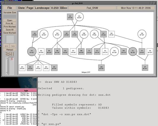
|
This macro first selects a pedigree or pedigrees named by the first argument of the macro (select temporarily subsets the dataset, and allows wild-card searches). It then calls the "write dot" command to create a file in the dot graphical language to draw the pedigree as a marriage node diagram. The circle (female) or square (male) representing an individual in the drawing will be shaded if that person is affected at the trait (the second argument to the macro). The "$" command allows two other programs to be called by Sib-pair, dot and gv (ghostview). Finally, the intermediate files are deleted, and all the other pedigrees returned to the list of active pedigrees.
The intermediate file names were created using the %% variable, which contains a (random) character string uniquely identifying the current macro call.
Macros can also be used as variables. The value of the macro is set using the macro command, but the contents are accessed using %<macro_name>". A macro variable can appear anywhere within a normal command.
>> macro a=1 >> macro b=+ >> %a%b%a => 2. >> macro a=D14S52 D14S43 >> tab %a ------------------------------------------------ Cross-tabulation of "D14S52" ... "D14S43" ------------------------------------------------ [...] |
When a macro is evaluated as a macro variable, macro positional parameters (%1, %2 etc) within the macro body are not evaluated.
This is another recent expansion of the language. Many Sib-pair commands automatically iterate over a class of eligible variables, for example the list of all active marker loci. In this case, the "keep" and "drop" commands can be used refine the selection.
For any command, a list of tokens enclosed in braces causes the command to be called repeatedly, substituting each member of the list into the command line at that location.
>> {1 2} + 1
=> 2.
=> 3.
>> tab { CHD carrier } ldl

------------------------------------------------
Cross-tabulation of "CHD" ... "ldl"
------------------------------------------------
                      ldl
CHD               1/1          1/2          2/2     Allele Freq  Exact HWE-P
           -----------------------------------------------------------------
     n         12 (.462)    11 (.423)     3 (.115)  0.6731  0.3269    1.0000
     y          0 (.000)     1 (1.00)     0 (.000)  0.5000  0.5000    1.0000
[...]
------------------------------------------------
Cross-tabulation of "carrier" ... "ldl"
------------------------------------------------
                      ldl
carrier           1/1          1/2          2/2     Allele Freq  Exact HWE-P
           -----------------------------------------------------------------
     n         24 (.774)     6 (.194)     1 (.032)  0.8710  0.1290    0.4027
     y          0 (.000)    13 (.867)     2 (.133)  0.4333  0.5667    0.0079

>> set loc a{1 2 3} aff; ls
a1* a2* a3*
 3  active traits;  0  active markers.
|
As can be seen in the last example, iteration is implemented in a macro fashion, and usually precedes evaluation of the other token. The exception to this is the handling of class summary tokens such as "$m" (all active autosomal markers) when they are the only value in the list. Multiple iteration and nested iteration are implemented.
>> 1{1 2} + {1 2}
=> 12.
=> 13.
=> 13.
=> 14.

>> 1{1 2 {3 4}}
=>  11.
=>  12.
=>  13.
=>  11.
=>  12.
=>  14.
|
Sib-pair can read in datasets in a variety of formats:
In addition, it can also merge data into existing pedigrees as a:
The simplest way to get data into Sib-pair is as in-lined data in a script. An example of such a script:
|
# declare four loci set locus a affection set locus b quantitative set locus m1 marker 0.0 cM set locus m2 marker 5.1 cM # read the pedigree data read pedigree inline # ped.id ind.id fa.id mo.id sex a b m11 m12 m21 m22 ex1 1a x x m n x 1 3 1 2 ex1 1b x x f n x 1 2 3 4 ex1 2a 1a 1b m n 3.5 1 2 1 3 ex1 2b x x f n 1.1 2 2 2 3 ex1 3a 2a 2b m y 4.3 1 2 1 2 ex1 3b 2a 2b m n 2.0 2 2 2 3 ex1 3c 2a 2b f n 0.8 2 2 3 3 ex1 4a 3c 3d f y x 1 2 2 3 ex1 3d x x m n x x x x x ex1 4b 3b 3e m y 4.7 1 2 3 4 ex1 4c 3b 3f m n 1.6 2 2 1 3 ;;;; # The four semicolons ends the in-line data run |
Pedigree data is comprised of one record (newline character delimited) per individual. Records should be sorted into pedigrees (though they can be joined subsequently with the "join" command). Records take the format used by GAS [Young 1995]:
pedigree-id person-id father-id mother-id sex-of-person locus-value-1...locus-value-N
A pedigree ID may be up to 20 alphanumeric characters, and an individual's personal ID up to 12 characters. Missing values are denoted x (or .), and represented internally as a trait value of -9999.
Locus values for a binary trait are y (expresses trait), n (does not express trait). Sex takes the values m (male) and f (female), and may be missing. Alleles at a marker locus are integers between 1 and 999 or single letters. The alleles of a genotype may be separated by a slash. A pedigree file may contain a comment at any time, prefaced by ! or #.
If only one parent of an individual is specified in the pedigree file, a dummy record and ID number for the other parent is generated by the program. Similarly, if both parental IDs are given, but there are no data records for those IDs, dummy records will be generated. A pedigree founder is a person where both parental ID fields (columns 3 and 4) are set to missing, and a nonfounder a person where both parental IDs are given.
>> set loc q1 qua >> set loc m1 mar >> read pedigree inline ped1 Bob Mark Alice m 10 a/b ;;;; >> run [Output omitted....] >> write Writing 1 pedigrees: ! ! S ! e !Ped Perso Fath Mothe x q1 m1 ! ped1 Alice x x f x x/x ped1 Mark x x m x x/x ped1 Bob Mark Alice m 10.0000 a/b |
As it happens, sex can also be coded as "1" (m) and "2" (f); binary traits as 1=n, 2=y.
A pedigree can either be read from a pedigree file (see below), or as in the example be inline in a script (or even entered from the keyboard). To read a script into Sib-pair, one can either send the contents of the script file directly to the program:
davidD@moonboom:~$ sib-pair < script.in |
or start up Sib-pair, and use the "include" command:
davidD@moonboom:~$ sib-pair |||| SIB-PAIR: A program for simple genetic analysis |\/| Version : F95-DEV (06-Nov-2006) |/\| Author : David L Duffy (c) 1995-2006 |||| Job run : Tue Nov 7 15:30:54 2006 >> include script.in |
If the "include" command is entered without specifying a file, a file chooser dialogue is opened. If "set gui" has been set, this is a graphical (AWT or GTK based) browser, but there is a backup text based browser:
>> include [1] ./ [2] ../ [3] cavanaughex.in [4] ex.in [5] ghex.in [6] linclex.in [7] liuex.in [8] longqtex.in [9] sib-pair.log [10] volgaex.in [11] williamsex.in choice> 7 Reading commands from "liuex.in". |
These dialogues allow one to change directory etc.
Finally, one can type in the commands and data interactively. This is most likely if you are going to simulate data:
>> set loc m1 marker >> sim ped 10 2 3 5 Simulating 10 pedigrees of depth 2 generations with sibship size 3 to 5 >> run |
This follows the same format as seen in the inline example. This could be prepared using a editor or a spreadsheet, saving the file as a plain text file (in Windows, a ".txt" file).
There needs to be a Sib-pair script that identifies the type of each column of data in the file, and the inclusion of the "read pedigree <file_name>" command:
>> set loc q1 qua >> set loc m1 mar >> read pedigree example.ped >> run |
There is also a Sib-pair native binary format, with associated "read bin" and "write bin" commands. This is written and read quickly. I would recommend reserving it for large datasets (eg genome-wide association scans), as it may not be portable across different operating systems, compilers etc. After saying this, I have not encountered this problem yet.
The Merlin pedigree file format is actually completely compatible with that used by Sib-pair except that alleles at a genotype in a Merlin type file must be numeric (a nonnumeric value for an allele is regarded as a missing value). The dataset columns can either be described using the "set locus" command, or alternatively the Merlin ".dat" locus description file could be read using the "read locus merlin <file_name>" command:
>> read locus merlin merlin.dat Read in names of 100 loci from locus file. >> read pedigree merlin.ped >> run |
Sib-pair can read both the "pre-makeped" and "post-makeped" Linkage format pedigree files. These are the formats used by a number of computer programs for genetic linkage and association analysis including the Linkage programs themselves (MLINK, ILINK, LINKMAP etc), Genehunter, Allegro, SUPERLINK, and UNPHASED. The full Linkage format is described online in several references.
Again, you can provide a description of the dataset columns using the "set locus" command, or read in the Linkage format ".dat" locus description file.
>> read locus linkage m_ger06.loc Read in names of 53 loci from locus file. >> read linkage m_ger06.pre >> run |
Plink genotype data files are either plain text or a compressed binary format (.bed). Sib-pair can read either style. For large datasets, it is a good idea to use the "compress" modifier, so that less memory is used.
The HapMap format is quite different from these other formats (individuals are columns, rows are genotypes), but again is read in fairly quickly.
>> read hap genotypes_chr15_CEU_r27_nr.b36_fwd.txt.gz
Pedigree file         = genotypes_chr15_CEU_r27_nr.b36_fwd.txt
Number of loci        = 108464
Number of individuals = 174
Number of genotypes   = 18872736
Read in  174 pedigrees, 174 individuals
         12671030 nonmissing SNP genotypes (31.15 s)
Dataset occupies 75.506 Mb.
|
VCF genotype data files are plain text (usually bgzip compressed) files that have become a standard for genotypes. Sib-pair has several functions for handling these - see the GWAS example below. Since VCF files do not record relationships between individuals, the merge vcf command is more useful.
As mentioned above, once a pedigree has been read into memory, extra data can be merged into previously declared variables. The merge command takes a file name, which can be preceded by an optional list of variables to select. The data to be merged can take the forms:
pedigree id trait1 geno1 geno2 A person1 y A/C 12/12 A person2 n x/x 10/12 ... |
Or if the individual IDs are unique,
id trait1 geno1 rs12312 person1 y A/C 12/12 person2 n x/x 10/12 ... |
Or, again if individual IDs are unique,
id locus allele1 allele2 person1 snp1 A C person1 strp1 10 12 person1 snp22 C C ... person2 snp1 C C ... |
Only the first four columns are read, so the rest of line (which might for example contain genotype quality score data) is discarded.
Merging data from other formats eg Plink are also straightforward.
Although there are a number of Sib-pair commands that can be used without having a dataset in memory, most are targetted at data analysis.
As already mentioned, this command declares a variable. Each "set locus" command declares the name and type of another column of data reading from left to right in the dataset.
>> set loc q1 qua >> set loc m1 mar |
The above two statements make the first data column (column 6 of the pedigree file) a quantitative trait called "q1", and second and third data columns (columns 7 and 8 of the pedigree file) the first and second alleles of an autosomal codominant locus called "m1".
The "set locus" declaration can be extended to give a genetic map position for the locus (in centiMorgans), and a 40 character comment describing the locus. Several commands can search the comments for particular strings (including wild card matches). For a trait as opposed to a marker, the position is usually unknown, but a place holder is needed if one wishes to write a comment.
>> set loc q1 qua . First quantitative locus >> set loc m1 mar 4.6 First marker locus >> list Locus Type Position --------------- ---- ---------- q1 q 6 First quantitative locus m1 m 7-- 8 First marker locus Number of marker loci= 1 Bonferroni corr. 5% = 0.050000 Bonferroni corr. 1% = 0.010000 Bonferroni corr. 0.1%= 0.001000 >> ls q1* m1 1 active traits; 1 active markers. |
The "list" command lists the currently declared loci in the dataset, while the "ls" command gives an abbreviated listing.
The listing can be limited to a subset of loci:
>> lis rs*00* Locus Type Position --------------- ---- ---------- rs1800420 m 286-- 287 rs1800420 25763792 G/G rs1800419 m 288-- 289 rs1800419 25770133 A/A rs1004611 m 290-- 291 rs1004611 25770873 - rs1800418 m 298-- 299 rs1800418 25789931 S/S rs1800417 m 300-- 301 rs1800417 25789974 I/T rs1800416 m 308-- 309 rs1800416 25844889 A/A Number of marker loci= 6 Bonferroni corr. 5% = 0.008512 Bonferroni corr. 1% = 0.001674 Bonferroni corr. 0.1%= 0.000167 >> lis $a Locus Type Position --------------- ---- ---------- cmm a 26 invasive a 36 |
Within the "list" command, loci selection can be via marker name, where matching can be by wildcards, or by locus type:
| $a | All active dichotomous traits |
|---|---|
| $q | All active quantitative trait |
| $h | All active haploid markers |
| $m | All active autosomal markers |
| $x | All active X-chromosome markers |
The latter can be further modified by addition of an ordering flag
| m | Genetic map order rather than column order |
|---|---|
| r | Reverse of column (or map mr) order |
The "run" command reads the pedigree data from the file (or script) into the dataset in memory. As it carries this out, it:
| Checks for duplicate records |
| Checks for impossible pedigree relationships (eg own father) |
| Checks sex of parents |
| Creates extra pedigree records as required |
| Sorts the pedigree by generation number |
| Checks for unconnected components within the pedigree |
| Tests and reports Mendelian errors |
| Tests that the reported sexes are consistent with sex-linked marker genotypes |
| Tests that monozygotic twins are concordant at all markers |
| Generates legal values for all missing genotypes within the pedigree - used to start MCMC algorithms. |
| Impute missing genotypes if requested ("set imputation on") |
Pedigree Individual Sex Post.Pr(M) X-marker hets ------------ ---------- --- ---------- -------------- 04620 0462030 f 1.000000 0/ 19 09901 0990151 f 1.000000 0/ 19 10157 1015704 m 0.000000 14/ 19 23204 2320403 m 0.000000 16/ 18 25122 2512203 m 0.000000 13/ 19 25122 2512204 f 1.000000 0/ 19 29344 2934401 f 1.000000 1/ 19 29344 2934450 m 0.000000 12/ 19 32802 3280203 m 0.000000 14/ 19 32802 3280204 f 1.000000 0/ 19 Designated Sex inferred via sex-linked markers Sex Likely Male Uncertain Likely Female ---------- ----------- --------- ------------- Male 721 1806 5 Unknown 0 145 0 Female 5 2136 811 |
The output from the testing of sex includes an estimate of the posterior probability an individual is male, if the probability of an inconsistency exceeds 99.9%. A count of the heterozygote genotypes for each person is also provided. If a sex informative marker such as amelogenin is available, this can be incorporated in the analysis.
NOTE:  inconsistency due child 34114-3411402 at locus GATA31F01P {145/153}

X-linked locus "GATA31F01P"
--------------
Sibship: 34114-3411403 x 34114-3411404

Inconsistency between sibling genotypes.

                      [3411403]           (3411404
                        x/-               145/153
                         |                   |
                         +=========+=========+
                                   |
               +---------+---------+---------+---------+
               |         |         |         |         |
            (3411401) (3411402) (3411451) [3411452] [3411453]
            145/149   145/153   145/153   153/-     153/-
|
Each Mendelian error detectable at a nuclear family level gives rise to a description of the individual where the error was detected, as well as a pedigree drawing showing all the relevant genotypes.
NOTE:  Mendelian inconsistency in pedigree 02590 at X-linked locus "GATA31E08".

X-linked locus "GATA31E08"
--------------
Sibship: 02590-0259001 x 02590-0000005

Multigenerational inconsistency between genotypes.

                 [0259003] (0259004)
                   x/-     242/242
                    |         |
                    +====+====+
                         |
                      [0259001]           (0000005
                        x/-                 x/x
                         |                   |
                         +=========+=========+
                                   |
                              +----+----+
                              |         |
                           [0259008] (0259009)
                           230/-     230/230

ID         Count    Problem phenosets
---------- -------- -----------------

Paternal Gparents
0259003           3 230/- 242/- +/-
0259004       Typed 242/242

Paternal Uncles/Aunts
0259002           1 242/-

Father
0259001     Problem 242/-

Mother
0000005     Problem 230/230 230/242 230/+ 242/242 242/+ +/+

Children
0259008       Typed 230/-
0259009       Typed 230/230

Parent 02590-0259001 cannot carry the "230" allele found in child 02590-0259008.
Parent 02590-0259001 cannot carry the "230" allele found in child 02590-0259008.
Parent 02590-0259001 cannot carry the "230" allele found in child 02590-0259009.
Parent 02590-0259001 cannot carry the "230" allele found in child 02590-0259009.
|
A multigenerational Mendelian inconsistency leads to printing of a table of pedigree members' observed or possible genotypes, along with (where possible) a statement of which transmission lead to the calling of the error. The pedigree drawing does not include uncles and aunts, so their genotypes must be found in the table. The above example is for a sex-linked marker.
If any errors are encountered during checking, the default action of the program is to stop. If the "set errordrop" command has been issued (on), then the pedigree, or the genotypes at the appropriate marker for the pedigree will be set to missing.
Usually, Sib-pair output goes to the screen in interactive mode. To save output, I usually run Sib-pair in batch mode from the command line, reading in a control script, and piping the output to a file:
> sib-pair < script.in > script.out |
During an interactive session, output can be diverted to a file by the "output" command. "output <filename>" saves subsequent output to the file filename, and "output" turns off the diversion, and resumes printing to the screen.
>> output script.out >> describe snps >> output |
This command produces summary statistics for the different variables. It can produce various amounts of output.
>> des snp Marker NAll Allele(s) Freq Het Ntyped -------------- ---- ----------- ------ ------ ------ rs977588 2 G (T) 0.4134 0.4851 3674 rs977589 2 A (G) 0.4548 0.4960 3818 rs2311843 2 A (G) 0.1474 0.2514 3815 rs1800415 1 G 1.0000 - 3828 rs7164127 1 C 1.0000 - 3828 rs1800414 2 G (A) 0.0034 0.0068 3828 |
The "describe snps" command produces a one-line summary for each marker giving the marker name, number of alleles, the allele names, the minor allele frequency if there are two alleles, the expected heterozygosity and number of individuals genotyped at that marker.
>> des rs977588

------------------------------------------------
Allele frequencies for locus "rs977588"
------------------------------------------------
   Allele  Frequency   Count  Histogram
     G       0.4134     3038  ********
     T       0.5866     4310  ************

Number of alleles    =    2
Heterozygosity (Hu)  =    0.4851
Poly. Inf. Content   =    0.3674
4 Neff mu (SSMM)     =    1.68136183
Number persons typed =   3674 ( 72.4%)
|
One obtains more information by not using the "snp" modifier.
For a quantitative trait, one would obtain,
>> des logIgE ------------------------------------------------ Summary statistics for trait "logIgE" ------------------------------------------------ Descriptive Stats All Founders Nonfounders ----------------------------------------------------- Means 4.4033 3.8716 4.6209 Variances 2.3192 1.8137 2.3647 Stand Devs 1.5229 1.3467 1.5378 Maxima 8.4338 8.3547 8.4338 Minima 2.0149 2.0149 2.0149 No. obs 1550 450 1100 No. missing 4076 2044 2032 |
-------------- Familial correlations (pairwise) -------------- Rel 1 Rel 2 Std Dev 1 Std Dev 2 Correlation N Pairs -------------------------------------------------------------- Husband Wife 1.2812 1.3113 0.0063 197 Gparent Gchild 0.0000 0.0000 0.0000 0 Halfsib Hsib 1.6126 -0.0417 19 Parent Off 1.3257 1.6067 0.2342 1208 Fullsib Fsib 1.5332 0.2986 967 Father Son 1.2363 1.5452 0.1765 273 Father Dau 1.2571 1.6201 0.1601 259 Mother Son 1.3900 1.5636 0.3145 356 Mother Dau 1.3673 1.6784 0.2448 320 Brothers 1.5042 0.3265 263 Sisters 1.5670 0.3937 313 Brother-Sister 1.4998 1.4969 0.1850 391 |
WLS estimates of heritability (approx SE) Heritability = 0.4662 (0.0008) Dominance (d2)= 0.2618 (0.0023) Fain sibship variance test -------------------------- No. sibships = 387 Intercept = 0.1031 (ase= 0.3792) Slope = -0.1242 (ase= 0.0793) t value = 1.5658 (df=385, P=0.0591) |
The results for a dichotomous trait are less extensive:
>> des hiIgE ------------------------------------------------ Segregation ratios for trait "hiIgE " ------------------------------------------------ Total sample All Fndrs Nonfndrs ------------------------------------------- Aff/Tot 686/1550 128/ 450 558/1100 Prop Aff 0.443 0.284 0.507 Missing 4076 2044 2032 Mating Type UxU UxA AxA ------------------------------------------- Matings 102 79 16 Aff/Tot 118/ 263 126/ 201 30/ 38 Prop Aff 0.449 0.627 0.789 Relative pair RecRisk Aff-Aff Aff-UnA ------------------------------------------- Marital 0.288 16 79 Gparent 0.000 0 0 Halfsib 0.769 10 6 Par-Off 0.459 230 542 Fullsib 0.625 312 375 |
The tables give the trait prevalence in founders, nonfounders and overall, the segregation ratios (unadjusted for ascertainment) -- the "davies" command gives adjusted estimates and standard errors, and the recurrence risks for different classes of relative pair.
The "set output" or "set plevel" command controls the verbosity of the printed output of the program. The usual level is "0", but it can be set both lower and higher than this. A plevel of "1" used to be standard, but this produces large amounts of output to be read. At that level, however, the details of the actual statistical tests performed are a lot clearer. Setting the plevel to "2" will give output from each iteration of an algorithm, such as likelihood maximization or simulation.
Setting the plevel to "-1" discards a number of warnings: Mendelian errors are reported as a single line of output per error, and minor pedigree problems (unrelated members etc) are not flagged.
The "hwe" command carries out a test for Hardy-Weinberg Equilibrium (HWE) on all (or a specified subset of markers). It calculates the likelihood ratio test statistic (LRTS) for HWE, but simulates P-values to allow for relatedness of pedigree members. All pedigree members therefore contribute to the test. This differs from the approach of several programs that test for HWE only in pedigree founders or unrelated individuals. The test is therefore a combined test of Hardy-Weinberg disequilibrium in founders and segregation distortion in nonfounders. The "founders" keyword restricts the analysis to founders only. And for diallelic markers, both the LRTS and HWE exact test P-values are calculated (the latter is only printed if plevel > 0).
>> hwe -------------------------------------------------- Hardy-Weinberg equilibrium for marker loci -------------------------------------------------- Marker Typed Genos Chi-square Asy P Emp P Iters ---------- ------ ------ ---------- ------ ------ ------ GATA52B03 1574 36 51.3 0.0368 0.0597 201 HWE + AGAT144 1562 36 28.0 0.7919 0.9524 21 HWE . GATA175D03 1499 78 53.6 0.9805 0.2273 88 HWE . ATA28C05 1538 28 26.4 0.4979 0.4651 43 HWE . GATA124E07 1598 120 112.7 0.6441 0.1439 139 HWE . GATA027 1569 21 12.9 0.8812 0.7143 28 HWE . GATA69C12 1585 36 27.1 0.8260 0.2941 68 HWE . GATA144D04 1519 55 51.6 0.5667 0.2985 67 HWE . GATA72E05 1534 36 29.1 0.7493 0.6452 31 HWE . GATA31D10 1577 36 34.5 0.4902 0.5882 34 HWE . GATA31F01 1580 66 62.6 0.5616 0.2500 80 HWE . GATA172D05 1589 36 37.2 0.3701 0.3846 52 HWE . GATA48H04 1538 36 18.3 0.9912 0.7407 27 HWE . GATA165B12 1590 15 26.5 0.0223 0.0249 201 HWE + ATCT003 1529 45 63.9 0.0267 0.0597 201 HWE + GATA31E08 1514 36 44.0 0.1421 0.3571 56 HWE . DXS998 1602 21 12.9 0.8802 0.7143 28 HWE . TATC043 1584 45 34.6 0.8431 0.4878 41 HWE . TTTA062 1587 21 40.5 0.0043 0.0448 201 HWE * |
>> set ple 1
>> hwe TTTA062

-> hwe TTTA062


--------------------------------------------------
Hardy-Weinberg equilibrium for marker loci
--------------------------------------------------

  -------- Observed Genotypes at "TTTA062   " --------
       Genotype          Observed    Expected  Deviate
  ----------------------------------------------------
        136/136          0 (0.000)        1.5     -1.6
        136/140          0 (0.000)        0.7     -1.0
        140/140          0 (0.000)        0.1     -0.2
        136/144         13 (0.015)        9.7      1.0
        140/144          3 (0.004)        2.4      0.5
        144/144         18 (0.021)       16.2      0.5
        136/148          6 (0.007)       12.1     -1.9
        140/148          5 (0.006)        3.0      1.1
        144/148         31 (0.036)       40.2     -1.5
        148/148         33 (0.039)       24.9      1.5
        136/152         55 (0.064)       41.3      2.0
        140/152          7 (0.008)       10.2     -1.0
        144/152        148 (0.173)      137.3      0.9
        148/152        171 (0.200)      170.4      0.1
        152/152        270 (0.316)      291.1     -1.2
        136/156          1 (0.001)        4.0     -1.7
        140/156          0 (0.000)        1.0     -1.2
        144/156          5 (0.006)       13.3     -2.7
        148/156         19 (0.022)       16.5      0.6
        152/156         65 (0.076)       56.4      1.1
        156/156          5 (0.006)        2.7      1.2
     Male Haplotype      Observed    Expected  Deviate
        136/-           26 (0.036)       30.3     -0.8
        140/-           10 (0.014)        7.5      0.9
        144/-          100 (0.137)      100.7     -0.0
        148/-          119 (0.163)      125.0     -0.5
        152/-          439 (0.600)      427.1      0.6
        156/-           38 (0.052)       41.4     -0.5
  ----------------------------------------------------
          Total       1587 (1.000)

       Number of genotypes =1587 ( 732 male)
  Hardy-Weinberg LR chi-sq =  40.5
Nominal degrees of freedom =  20
           Nominal P-value =   0.0043
      Equalled or exceeded by =   7/  201 simulated values (0.0348)
 Mean (Var) simulated chi-sqs =  24.1 (  66.7)
|
In this example, the markers are X-linked, so the test includes a contribution due to allele frequencies differences between males and females. There are two sets of P-value, the asymptotic P-values ignoring relationships and the empirical P-values obtained from gene-dropping using the observed pedigree structure and allele frequencies. The "Iters" column (and the equivalent line in the verbose output) gives the number of simulations (replicates of the dataset) used. The maximum number of simulations defaults to 200, but if the P-value is nonsignificant, the sequential approach used will stop early.
The other test for HWE that Sib-pair provides compares the observed to expected heterozygosities:
>> homoz -------------------------------------------------- Marker homozygosity in all typed individuals -------------------------------------------------- Marker N Obs Exp Fis Z Emp P Iters ---------- ---- ------ ------ ------ ------ ------ ------ TTTA062 855 0.3813 0.3936 -.0203 -0.7 0.6452 31 HOM . |
This command, "homoz" can also be applied to homozygosity mapping or Hardy-Weiberg disequilibrium mapping by specifying a dichotomous trait: "homoz <trait>".
Finally, use of the "table" command to crosstabulate a diallelic marker by another locus gives an exact HWE test for each stratum.
>> tab q1 rs8004738

------------------------------------------------
Cross-tabulation of "q1" ... "rs8004738"
------------------------------------------------

                      rs8004738
q1                C/C          C/T          T/T     Allele Freq  Exact HWE-P
           -----------------------------------------------------------------
   1.00000    271 (.230)   620 (.527)   285 (.242)  0.4940  0.5060    0.0705
   2.00000    151 (.227)   342 (.515)   171 (.258)  0.4849  0.5151    0.4383
|
There are several Sib-pair commands that can be used to transform the pedigree structure of a dataset. The simplest such command ("nuclear") breaks down a larger pedigree into its constituent nuclear families:
>> nuc Dividing pedigrees into nuclear families. Individuals are duplicated as necessary. Reread 16 pedigrees, 90 individuals (0.00 s). Dataset occupies 0.010 Mb. Extracted 16 nuclear families. |
The "grandparents" modifier adds in the grandparents for each nuclear family, such that they will be "CEPH" type families.
Another command for pedigree manipulation is "join" which connects pedigrees together via common individual IDs. This is useful if you wish to reconnect subsets of nuclear families created using the "nuclear" command. Thus you can subdivide a pedigree into the largest blocks analyzable by another program; such as MERLIN.
The other commands for pedigree manipulation include "prune", which removes pedigree members who are uninformative for a particular trait locus (unknown status themselves, and not connecting informative sets of relatives); and "case" which extracts the unrelated cases and controls from a pedigree, discarding other pedigree members.
While the "keep|drop" and "undrop" commands allow you to choose the subset of data columns -- ie variables, the "select" and "unselect" commands allow the selection of rows of data -- pedigrees. Selection is either by the desired pedigree names, or using a "where" clause; which can be any logical expression.
>> select containing 2 where anytyp Selecting pedigrees to contain 2 or more individuals where "anytyp": Number of pedigrees selected= 15 ( 334 individuals) |
The previous command selected only those pedigrees where two or more members are genotyped at any active marker (we could have used the "keep|drop" command to restrict the test to a subset of all the markers). If genotyping is patchy, we might have instead used:
>> unselect >> select containing 2 where commar > 2 |
where commar is a function counting the maximum number of markers an individual shares with any of their relatives.
This can be between markers (linkage disequilibrium, LD) or between a trait locus and a marker.
The "disequilibrium" command defaults to calculating measures of linkage disequilibrium for pairs of codominant marker loci. It tests both intragametic and intergametic association.
>> dis 2 2
  9 genotype counts>
91 147 85
32 78 75
5 17 7
Modelling   9 unphased genotypes (N=  537).

  Haplotype  Prop      95% CL           D        D'
  ----------------------------------------------------
   1   1   0.3822   0.3503--0.4169    0.0234    0.2231
   1   2   0.3916   0.3594--0.4266   -0.0234   -0.2231
   2   1   0.0815   0.0664--0.1001   -0.0234   -0.2231
   2   2   0.1448   0.1244--0.1684    0.0234    0.2231

  Number of genotypes used =       537
    LD Model LR Chi-square =       12.81 (df=   5, P=0.0252)
       LR Chi-square (D=0) =        8.01 (df=   1, P=0.0046)
  Hedrick weighted mean D' =        0.2231
                 r-squared =        0.0126
|
This analysis read a 3x3 table of genotype counts from the command line -- the "dis 2 2" lead Sib-pair to expect data for two diallelic markers. Sib-pair fitted loglinear models to the counts, the critical one allowing linkage disequilbrium between the two loci (D' > 0). It tested this model against that assuming complete linkage equilibrium, giving a significant LRTS=8.01. Since these are both diallelic markers, Sib-pair also printed the r2 measure of LD as well as D'.
For family data, Sib-pair uses parents where available to infer haplotype phase, and combines information from phased and unphased genotypes. Pedigree members are discarded as appropriate, so that the resulting tables of genotype counts come from unrelated individuals.
>>  set ple 2
>>  dis A308G rs3897937

->  dis A308G rs3897937


---------------------------------------------------
Inter-marker allelic association analysis
---------------------------------------------------


Assoc for locus "A308G     " c. locus "rs3897937 "
---------------------------------------------------

Modelling  10 phased genotypes (N=  319) and   9 unphased genotypes (N= 1619).
And   4 male haplotypes (N= 1360).

Unphased Genotypes  Observed  Expected  Deviance
  1/1     1/1           774.    769.2      0.2
  1/1     1/2           495.    503.0     -0.3
  1/1     2/2           101.     82.2      2.0
  1/2     1/1             0.      0.0     -0.0
  1/2     1/2           175.    190.5     -1.1
  1/2     2/2            55.     62.3     -0.9
  2/2     1/1             0.      0.0      0.0
  2/2     1/2             0.      0.0     -0.0
  2/2     2/2            19.     11.8      1.9
Phased Genotypes    Observed  Expected  Deviance
  1  1;  1  1           149.    151.6     -0.2
  1  1;  2  1           100.     99.1      0.1
  1  1;  2  2            21.     16.2      1.2
  2  1;  1  1             0.      0.0     -0.0
  2  1;  1  2             0.      0.0     -0.0
  2  2;  1  1             0.      0.0      0.0
  2  1;  2  1            41.     37.5      0.6
  2  1;  2  2             8.     12.3     -1.2
  2  2;  2  1             0.      0.0     -0.0
  2  2;  2  2             0.      2.3     -2.2
Male Haplotypes     Observed  Expected  Deviance
     1 1                952.    937.4      0.5
     1 2                278.    306.5     -1.7
     2 1                  0.      0.0     -0.0
     2 2                130.    116.1      1.3

  Haplotype  Prop      95% CL           D        D'
  ----------------------------------------------------
 A   A     0.6893   0.6686--0.7105    0.0588    1.0000
 A   G     0.2254   0.2131--0.2383   -0.0588   -1.0000
 G   A     0.0000   0.0000--  +Inf   -0.0588   -1.0000
 G   G     0.0854   0.0779--0.0936    0.0588    1.0000

  Number of genotypes used =      3298
    LD Model LR Chi-square =       22.61 (df=  17, P=0.1622)
       LR Chi-square (D=0) =      898.94 (df=   1, P=0.0000)
  Hedrick weighted mean D' =        1.0000
                 r-squared =        0.2070
|
In this example, the SNPs are on the X-chromosome, so males provide haplotype frequencies directly, but no information about intergametic association. There is "complete" LD, but not "perfect" LD. The overall model goodness-of-fit test is not significant, thus suggesting an absence of intergametic effects.
If one specifies the names of more than two autosomal markers, or two or more autosomal markers and a binary trait, then the command estimates haplotype frequencies using a log-linear model.
>> dis G2215A ACE_ID G2350A hiace

---------------------------------------------------
Inter-marker allelic association analysis
---------------------------------------------------

Trait:   hiace(2)
Markers: G2215A(2) ACE_ID(2) G2350A(2)

Haplotype  n           y
--------   ---------   ---------
1 1 1      0.0000      0.0000
2 1 1      0.6711      0.2975
1 2 1      0.0000      0.0000
2 2 1      0.0000      0.0000
1 1 2      0.0000      0.0000
2 1 2      0.0000      0.0000
1 2 2      0.3263      0.6994
2 2 2      0.0026      0.0032

hiace         190         158

            Number of loci =         3
 No. genotyped individuals =       348
 No. obs. unique genotypes =         8
  Stratified LD Chi-square =        18.26 (df=  48, P=1.0000)
    Association Chi-square =        98.91 (df=   2, P=0.0000)

NOTE:  Degrees of freedom calculation for association test assumes only
          3 haplotypes to be present in the population.
|
The algorithm used is not optimized for either large numbers of alleles or large numbers of loci.
There are six specialized trait locus association commands:
| assoc | Total association; FBAT (Family-based Association Test) |
| mgt | Variance components based likelihood ratio test |
| mqls | Quasi-likelihood tests for binary trait association in pedigrees |
| mqls | WQLS quasi-likelihood test |
| tdt | Transmission-disequilibrium tests |
| hrr | Haplotype relative risk test |
| schaid | Schaid's TDT |
| sdt | Sibship disequilibrium test |
These are supplemented by the "regression" command, which also allows gene-dropping for pedigrees (via the simulate modifier), and commands for "measured genotype" models -- "varcom" and "fpm". The "mgt" command is a simple front end to "varcom". And as noted above, the "homoz" command can also be a powerful test of association in a case-only analysis.
The "assoc" command and regression tests can be used for samples of unrelated individuals and family data. They deal with familial correlated data by calculating gene-dropping simulated P-values. The type of gene-dropping currently used is not conditional on marker IBD, so although the resulting test has the correct size in a statistical sense, it can detect linkage as well as pure association in larger pedigrees:
>> ass AD -------------------------------------------------- Allelic association testing for trait "AD" -------------------------------------------------- Marker Typed Allels Chi-square Asy P Emp P Iters ---------- ------ ------ ---------- ------ ------ ------ D14S52 21 7 4.7 0.5890 0.2793 179 AssX2-HWE . D14S52 6 7 0.5 1.0000 0.8772 57 RC-TDT . D14S43 21 7 12.6 0.0498 0.0064 5001 AssX2-HWE * D14S43 2 7 2.9 0.5171 0.2404 208 RC-TDT . D14S53 20 6 11.0 0.0516 0.0054 5001 AssX2-HWE * D14S53 3 6 1.0 1.0000 0.4237 118 RC-TDT . |
These results are from three Volga German Alzheimer's pedigrees described in Figure 1 of Schellenberg et al [1992]. These families harbour mutations in the presenilin 1 gene. At 72.673 Mbp from the pter of chromosome 14, this is 1.34 Mbp from D14S43, (the closest of the three microsatellite markers used in that paper), which gave a linkage lod score of 7.
>> keep AD D14S43
>> select pedigree L
>> set iterations 90000
>> set plevel 1
>> assoc AD
--------------------------------------------------
Allelic association testing for trait "AD"
--------------------------------------------------

  ---- Association Analysis for "D14S43    "-----
    Allele   Affected    Unaffected    Total    Dev
  ------------------------------------------------
   159       11 (.786)      0 (.000)      11    2.3
   179        0 (.000)      1 (.167)       1   -1.5
   181        2 (.143)      1 (.167)       3   -0.2
   183        1 (.071)      0 (.000)       1    0.7
   185        0 (.000)      2 (.333)       2   -3.1
   187        0 (.000)      2 (.333)       2   -3.1
  -------------------------------------------------
   Total     14             6             20

       No. trait(+) marker(-) =    20
       No. trait(+) marker(+) =    10
                Fis, Fit, Fst =   -.1765   0.2683   0.3780
   Contingency Pearson chi-sq =  16.8
   Nominal degrees of freedom =   5
              Nominal P-value =   0.0048
      Equalled or exceeded by =   4/90001 simulated values (0.0000)
 Mean (Var) simulated chi-sqs =   2.8 (   4.5)
|
We can obtain a more impressive result by restricting our analysis to one pedigree (pedigree L), where the 159 allele cosegregates with the disease. The point is that we are observing a pure test of cosegregation/linkage, that is correctly modelling the transmission of the marker allele through the pedigree.
By contrast, in the study of Liu et al [1996], 15 late-onset Alzheimer's pedigrees were genotyped at the APOE locus. Evidence of linkage to APOE was weak, but there was strong evidence of allelic association.
>> ass AD -------------------------------------------------- Allelic association testing for trait "ad" -------------------------------------------------- Marker Typed Allels Chi-square Asy P Emp P Iters ---------- ------ ------ ---------- ------ ------ ------ apoe 163 3 18.4 0.0001 0.0001 50001 AssX2-HWE *** |
Since there are few alleles (and the result was strongly significant), it is worth looking at the genotypic effects.
>> set plevel 1
>> ass AD gen

-> ass ad gen

--------------------------------------------------
Allelic association testing for trait "ad"
--------------------------------------------------
NOTE:  Genotypic rather than allelic association test.

  ---- Association Analysis for "apoe      "-----
  Genotype   Affected    Unaffected    Total    Dev
  ------------------------------------------------
   2/2        0 (.000)      0 (.000)       0    0.0
   2/3        1 (.023)      7 (.058)       8   -1.0
   3/3        7 (.163)     58 (.483)      65   -2.9
   2/4        1 (.023)      5 (.042)       6   -0.6
   3/4       23 (.535)     38 (.317)      61    2.0
   4/4       11 (.256)     12 (.100)      23    2.4
  -------------------------------------------------
   Total     43           120            163

       No. trait(+) marker(-) =   168
       No. trait(+) marker(+) =    81
   Contingency Pearson chi-sq =  18.7
   Nominal degrees of freedom =   4
              Nominal P-value =   0.0009
      Equalled or exceeded by =  20/28061 simulated values (0.0007)
 Mean (Var) simulated chi-sqs =   4.1 (   7.6)
|
The genotypic test simulation P-value is also highly significant. The greatest risk of disease was associated with the APOE*E3/APOE*E4 and APOE*E4/APOE*E4 genotypes
The MQLS test of Thornton and McPeek [2007] also gives an impressively significant result. This test is a bit more approximate (as it relies on several assumptions), especially in large pedigrees, but is much faster for screening large numbers of markers for association.
>> set plevel 0 >> mqls ad -------------------------------------------------- MQLS association testing for trait "ad" -------------------------------------------------- Marker Typed Allels Chi-square Asy P -------------- ------ ------ ---------- ------ apoe 166 3 18.0 1e-5 MQLS *** |
Increasing the plevel will cause all three quasi-likelihood statistics to be printed out for each allele in turn. The MQLS requires an acceptable estimate of the trait prevalence, and in this small dataset, the "Best Linear Unbiased" estimates for the allele frequencies can end up negative for alleles where there is little information.
>> set plevel 0 >> mqls ad 0.05 -------------------------------------------------- MQLS association testing for trait "ad" -------------------------------------------------- Trait model prevalence = 0.0500 MQLS results for: apoe Allele Case Freq E(Freq) SD Z Value P-value ------- ---------- ------- ------- -------- ------- 2 0.0135 0.0514 0.0307 -1.23 0.2183 MQLS 2 -0.1984 0.0514 0.1713 -1.46 0.1448 WQLS 2 0.0233 0.0422 0.0190 -1.00 0.3185 corrX2 3 0.3958 0.6388 0.0669 -3.63 0.0003 MQLS 3 -0.6554 0.6388 0.3726 -3.47 0.0005 WQLS 3 0.4419 0.6114 0.0413 -4.11 4e-5 corrX2 4 0.5907 0.3098 0.0644 4.36 1e-5 MQLS 4 1.8538 0.3098 0.3587 4.30 2e-5 WQLS 4 0.5349 0.3464 0.0397 4.75 2e-6 corrX2 |
>> surv onset AD apoe

------------------------------------------------------
Nonparametric survival analysis of trait "onset"
------------------------------------------------------
"ad" is outcome (censoring) trait.
Covariates: apoe

Number of strata         = 5
Number of distinct times = 51

                                 ad
   apoe             N       Obs       Exp       Var       Z
---------- --------------------------------------------------
    2/3             8         1      2.35      2.09     -0.93
    2/4             6         1      3.00      2.54     -1.26
    3/3            64         7     18.69      9.49     -3.79
    3/4            61        23     13.82      8.65      3.12
    4/4            23        11      5.14      4.16      2.87

Log-rank Chi-square=  24.93 df=  4 (P=5e-5)
|
It is possible to carry out a nonparametric survival analysis (see above Table) on the ages-at-onset in this set of pedigrees and confirm the association. Note that this result does not incorporate an adjustment for residual familial correlation, and so may be too generous in this example.
Rerunning the command without specifying the marker locus obtains a gene-dropping P-value for all active loci:
>> set plevel 0 >> set iter 10000 >> surv onset AD ------------------------------------------------------ Nonparametric survival analysis of trait "onset" ------------------------------------------------------ "ad" is outcome (censoring) trait. Marker Nobs NAff Chi-square Asy P Emp P Iters -------------- ------ ------ ---------- ------ ------ ------ apoe 162 43 24.9 5e-5 0.0098 2040 Surv *** |
>> regress onset = apoe weibull AD sim

------------------------------------------------
Weibull  regression analysis of trait "onset"
------------------------------------------------
Censoring variable: ad.

    Variable         Beta    Stand Error        t-Value
  -----------------------------------------------------
  Intercept       43.6621         1.4266        30.6064 ***
  apoe*3          -0.7437         0.7265         1.0237 .
  apoe*4          -1.8245         0.7385         2.4705 *

No. usable observations =    162      ( 48.5%)
No. of uncensored times =     43      ( 26.5%)

Weibull shape parameter =      9.4276
Number of iterations    =     91
Model LR Chi-square     =    111.5137 (df= 159)
Akaike Inf. Criterion   =    117.5137

ERROR: IRLS failed (perhaps due to separation).

Due to IRLS failure, discarded Pseudosample      128

Gene-dropping association test for "apoe"
Equalled or exceeded by =    1/ 50001 simulated values (0.0000)
Mean (Var) sim deviance =    123.6625 (      1.9032)
|
We can also carry out a Weibull-regression based survival analysis (see above Table) on the ages-at-onset in this set of pedigrees and confirm the association. Out of over 50000 simulations, about 50 give an error message (probably due to one or more genotypes not appearing in cases or controls) -- these were discarded and replacement samples drawn.
An alternative approach is to generate residuals from a survival analysis and carry out association analysis on these:
>> set loc adres qua Creating new variable "adres". >> adres=onset Operating on pedigree file Recoded 165 values. >> kap adres ad res |
------------------------------------------------
Kaplan-Meier survivor function for "adres"
------------------------------------------------
"ad" is outcome (censoring) trait.

Replacing value of "adres" with nonparametric residual.

 Age-at-onset   Failed  Riskset   H(t)   S(t)    ase
 ---------------------------------------------------
      52.0000        1      111 0.0090 0.9910 0.0090
      57.0000        1       98 0.0192 0.9809 0.0134
      58.0000        1       95 0.0297 0.9706 0.0168
      59.0000        1       94 0.0404 0.9602 0.0195
      60.0000        4       91 0.0843 0.9180 0.0278
      61.0000        2       84 0.1081 0.8962 0.0312
      62.0000        1       79 0.1208 0.8848 0.0328
      65.0000        5       74 0.1884 0.8250 0.0400
      67.0000        4       66 0.2490 0.7750 0.0447
      68.0000        1       58 0.2662 0.7617 0.0459
      69.0000        3       56 0.3198 0.7209 0.0491
      70.0000        4       50 0.3998 0.6632 0.0530
      72.0000        5       37 0.5349 0.5736 0.0591
      73.0000        1       30 0.5683 0.5545 0.0601
      76.0000        5       24 0.7766 0.4389 0.0662
      79.0000        2       15 0.9099 0.3804 0.0691
      80.0000        1       12 0.9933 0.3487 0.0702
      83.0000        1        7 1.1361 0.2989 0.0758

 H(t) = Nelson-Aalen estimator of integrated hazard
 S(t) = Kaplan-Meier estimator of survivor function

   43 affecteds and   122 unaffecteds used

>> ass adres gen

>> ass adres gen


--------------------------------------------------
Allelic association testing for trait "adres"
--------------------------------------------------
NOTE:  Genotypic rather than allelic association test.

  ------ QTL Association with "apoe      " -----
  Genotype   Gtypic Mean     Stand Error   Count
  ----------------------------------------------
   2/2             0.0000         0.0000       0
   2/3            -0.3562         0.2815       8
   3/3            -0.3421         0.0988      65
   2/4            -0.6132         0.3250       6
   3/4             0.1996         0.1003      63
   4/4             0.3937         0.1660      23
  ----------------------------------------------
  Total           -0.0433         0.8485     165

 No. trait(+) marker(-)  =      0
 No. trait(+) marker(+)  =    165
 Model Mean Square       =      3.3907 (df=   5)
 Mean Square Error       =      0.6339 (df= 160)
 Likelihood ratio test   =     25.0743
 Nominal P-value         =      0.0000
 Equalled or exceeded by =   3/50001 simulated values (0.0001)
 Mean (SD) simulated MSE =      0.7222 (      0.0114)
|
In the table above, the use of Sib-pair's "kaplan-meier" command provides the Kaplan-Meier estimate of the survival curve, as well as replacing the age-at-onset trait by the transformed martingale residuals if the "residuals" keyword is included. A standard ANOVA is performed, and gene-dropping used to give a correct P-value given the relatedness of the sample. Even after transformation (following Therneau), the residuals are not "nicely" distributed, so the gene-dropping is doubly necessary.
>> his adres

------------------------------------------------
Mixture distributions for trait "adres"
------------------------------------------------

 Intvl Midpt  Count   Histogram
 -------------------------------------------------------
     -1.4066     11   ***********
     -1.2463      4   ****
     -1.0033      7   *******
     -0.8016     17   *****************
     -0.6138      3 | ***
     -0.3984     10 | **********
     -0.1967     17 | *****************
      0.0049     57 + **************************************************
      0.2426      5   *****
      0.4082      0
      0.6099      6   ******
      0.7957      4   ****
      1.0131      4   ****
      1.2148      9   *********
      1.4164      0
      1.6181      3   ***
      1.7648      4   ****
      2.1213      1   *
      2.2561      1   *
      2.4378      1   *
      2.7271      1   *

Filliben correlation =        0.8037 (P=0.000)

Poissonness test Z   =     -582.9685 (P=1.000)
Median (IQR)         =        0.0000 (      -0.6138 --        0.0068)
Symmetry test J(.02) =        0.4142 (P=0.000)
|
Association analysis using the " regress" or "fpm" commands can also include inferred marker genotypes for untyped members of the pedigree via two different methods. One can estimate the expected gene dose for the marker using the "gpe" command, and use this instead of the observed genotypes in the regression. This does not allow for residual family correlation (unless "fpm" is used).
Alternatively, by issuing the "set analysis imputed" command, each subsequent "regress" call will cause reimputation of missing genotypes (at the marker included in the model), with these imputed genotypes being included in the regression analysis. It is then necessary to fit the model repeatedly and average over test statistics (multiple imputation) so as to correctly represent the uncertainty in the estimates for the unobserved genotypes. This is carried out automatically by the replicates option of the "regress" command.
Tests such as the transmission-disequilibrium test (TDT), and the Family-based Association test (FBAT) are tests of joint linkage and association. In practice, they are usually seen as association tests that are insensitive to confounding due to ethnic stratification in a sample of families. Sib-pair automatically performs a simulation-based version of the FBAT whenever the "assoc" command is run. The gene-dropping is performed conditional on parental genotypes (CPG) and conditional on offspring genotypes needed to impute missing parental genotypes.
>> inc liuex.in >> set plevel 1 >> ass AD -> ass ad |
Returning to the dataset from Liu et al [1996], we obtain:
 -------- Combined transmission test for "      apoe" --------
   Allele   Affected   Unaffected   Total   E(Aff)    Z    P
 -------------------------------------------------------------
     2        2 (.03)      6 (.10)      8    3.7   -1.3 0.1830
     3       28 (.41)     37 (.60)     65   34.5   -2.2 0.0306
     4       38 (.56)     19 (.31)     57   29.8    2.7 0.0073
 -------------------------------------------------------------
   Total     68           62          130

                    marker(-) =     3
       No. trait(+) marker(+) =    65
          No. useful sibships =    13
 Global association statistic =   2.2
           Degrees of freedom =   2
      Equalled or exceeded by =  20/ 1349 simulated values (0.0148)
 Mean (Var) simulated chi-sqs =   0.5 (   0.3)
|
The second column records the number of times that the different alleles were transmitted from a parent to an affected child. The third column records the number of times the same alleles were transmitted to an unaffected child. Since the latter does not usually contribute much information, only the affected transmissions are used to construct the score test, where "E(Aff)" is the number expected under the null hypothesis of no association. The unaffecteds are used to help impute missing parental alleles. Both "E(Aff)" and "SD(Aff)" are produced by a gene-dropping (with rejection sampling) algorithm. Using these simulated values, a Z statistic for over/undertransmission of each allele is calculated, and the asymptotic P-value for this statistic.
In this example, the overtransmission of the APOE*4 allele to Alzheimer's disease cases is the largest single contribution. Sib-pair combines the statistics from the alleles into a global test for which a simulation based P-value is produced. If the "plevel"=2, one obtains:
--------- Sibships used for RC-TDT --------------------
Pedigree       Father         Mother      Aff Tot
F102              204 (2/3)    203 (2/2)   1   3  2/3
F106              101 (2/3)    102 (1/3)   4   5  2/3 1/3 3/3 2/3
F107              101 (2/3)    102 (2/3)   4   8  2/3 2/3 3/3 2/3
F118              101 (2/3)    102 (x/3)   2   3  3/3 3/3
F133              203 (1/3)    204 (2/3)   1   4  3/3
F133              202 (x/2)    201 (2/3)   1   2  2/3
F151              101 (x/2)    102 (2/3)   3   7  2/2 2/3 2/3
F163              101 (x/2)    102 (2/3)   4   6  2/3 2/2 2/3 2/3
F164              101 (x/2)    102 (2/3)   2   6  2/3 2/3
F175              201 (1/2)    202 (2/3)   3   6  1/2 2/2 2/2
F176              201 (2/3)    202 (x/3)   3   7  3/3 3/3 3/3
F197              101 (x/2)    102 (2/3)   3   6  2/3 2/2 2/3
F204              101 (2/3)    102 (x/3)   3   5  3/3 3/3 2/3


  Allele     Tr   E(Tr)  Cov(Tr)
 ------- ------ ------- --------------------------------------
     2        2    3.74    1.71
     3       28   34.45   -0.59    9.24
     4       38   29.80   -1.13   -8.65    9.78

  Parents genotyped   No. Fams  Useable  Aff Off
 ------------------   --------  -------  -------
  None                      24       12       33
  Father only                4        0        0
  Mother only               20        1        1
  Both parents              12        0        0
|
The "tdt" command performs the classical TDT of Spielman et al [1993], each allele versus all others, two multiallelic TDTs, and a genotypic TDT.
Here is an example using the TDT to fine map the Finnish late infantile neuronal ceroid lipofuscinosis gene (CLN5) in Finnish families segregating this rare Mendelian disorder (as per Figure 1 of Savukoski et al 1994).
>> include linclex.in >> tdt oneperfam ------------------------------------------------ TDT for trait "oneperfam" v. all markers ------------------------------------------------ Marker Typed NParam Chi-square Asy P Emp P Iters ---------- ------ ------ ---------- ------ ------ ------ D13S162 10 8 11.3 0.0068 0.0068 0 TDT-Best * D13S162 10 8 13.0 0.1118 0.0509 393 TDT-All + D13S162 10 7 19.8 0.0061 0.0061 0 TDT-Ewens * D13S162 10 2 15.0 0.0006 0.0398 201 TDT-Gtp ** D13S160 10 6 16.0 0.0002 0.0002 0 TDT-Best ** D13S160 10 7 18.0 0.0120 0.0005 2001 TDT-All ** D13S160 10 5 25.6 0.0001 0.0001 0 TDT-Ewens ** D13S160 10 1 20.6 0.0000 0.0100 201 TDT-Gtp *** D13S170 8 11 3.6 1.0000 1.0000 0 TDT-Best . D13S170 8 11 14.0 0.2330 0.0545 367 TDT-All + D13S170 8 10 14.2 0.1649 0.1649 0 TDT-Ewens . D13S170 8 4 15.0 0.0047 0.2564 78 TDT-Gtp * |
The best results seem to be for D13S160.
>> keep oneperfam D13S160 >> set plevel 1 >> tdt oneperfam |
So we will examine the detailed output.
------------------------------------------------
TDT for trait "oneperfam" v. all markers
------------------------------------------------

Number of informative probands:  10

  - Allele by Allele TDT:"D13S160   " -
  Allele   Trans  Not Tr   TDT   P-value
  --------------------------------------
     1         2       4   0.7    0.6875
     2         0       6   6.0    0.0313
     3         0       3   3.0    0.2500
     4         0       4   4.0    0.1250
     5        16       0  16.0    0.0000
     6         0       1   1.0    1.0000

No. of alleles used  =    6
Bonferroni corr. 5%  =    0.010206
Bonferroni corr. 1%  =    0.002008
Bonferroni corr. 0.1%=    0.000200
|
The first table gives a TDT for each allele (versus all others). Heterozygous parents transmitted the "5" allele on 16 occasions, and it was never the nontransmitted allele. The fourth column is the TDT Chi-square, but the fifth column is the binomial exact P-value, but unadjusted for multiple testing (of 6 alleles).
In the summary table generated when plevel=0, the result for the best allele (allele 5) was given as "TDT-best", and the P-value was Bonferroni corrected.
  -------- Global Allelic TDT --------
   All 1   All 2    Tr=1    Tr=2   TDT
  ------------------------------------
     1       2         1       0   1.0
     1       4         1       0   1.0
     1       5         0       4   4.0
     2       5         0       5   5.0
     3       5         0       3   3.0
     4       5         0       3   3.0
     5       6         1       0   1.0

Allelic TDT Pearson chi-square=  18.0
            Degrees of freedom=   7
                       P-value=   0.0120
Empiric P-value (   2001 iter)=   0.0010

  Ewens allelic TDT chi-square=  25.6
            Degrees of freedom=   5
                       P-value=   0.0001
|
The next two tests are multiallelic TDTs. The table gives the pattern of transmission from each heterozygous parent to an affected child -- for example, there were 5 parents carrying the "2/5" genotype, and in each case the "5" allele was transmitted. The asymptotic P-value for this relatively sparse table is too conservative (P=0.012). By contrast, the empirical P-value, generated by permutation, is more impressive.
The Ewens test combines the six allelic TDT Chi-squares together into a (generally) more powerful multiallelic test.
  ----- Genotypic Transmission Test ------
       Genotype     Trans  Expected   Dev
  ----------------------------------------
          1/2          0       0.5   -0.7
          1/3          0       0.5   -0.7
          1/4          0       0.2   -0.4
          1/5          2       1.5    0.5
          1/6          0       0.2   -0.4
          2/3          0       0.2   -0.4
          2/4          0       1.0   -1.2
          2/5          0       1.2   -1.4
          3/5          0       0.8   -1.0
          4/5          0       0.8   -1.0
          5/5          7       1.8    2.6
          5/6          0       0.2   -0.4

Genotypic Transmission Chi-sq =  20.6
   Nominal degrees of freedom =   1
              Nominal P-value =   0.0000
      Equalled or exceeded by =   2/ 201 simulated values (0.0100)
Mean of simulated chi-squares =  10.8
|
Finally, the genotypic TDT is similar in flavour to the FBAT statistic in calculating the expected number of each genotype given the set of parental genotypes (mating types). It uses a CPG gene-dropping to assess significance. Because there are more genotypes than alleles, it is usually a less powerful test than an allelic TDT.
An alternative genotypic TDT is the loglinear model described by Schaid and Sommer [1993].
>>>> schaid oneperfam D13S160 5

--------------------------------------------------
Schaid & Sommer analysis of trait "oneperfam"
--------------------------------------------------
Versus allele   5 of marker D13S160

------------------------------------------------------------
      Mating         Total Expected   5/5     5/-     -/-
------------------------------------------------------------
  5/5   x   5/5          0      0.4     0       x       x
  5/5   x   5/-          0      2.0     0       0       x
  5/5   x   -/-          0      1.2     x       0       x
  5/-   x   5/-          8      2.5     7       1       0
  5/-   x   -/-          2      3.0     x       2       0
  -/-   x   -/-          0      8.1     x       x       0
------------------------------------------------------------

Freq of   5 allele   =     0.050
N affected children  =    10

HWE Chi-square (2 df)=    30.73 (P=0.000)
Genotypic RR1 (f1)   = 11044.69 (95%CI=    0.00 to ********)
Genotypic RR2 (f2)   = ******** (95%CI=    0.00 to ********)
Attributable risk    =     1.00

CPG Chi-sq    (2 df) =    17.54 (P=0.000)
Genotypic RR1 (f1)   =   943.19 (95%CI=    0.00 to ********)
Genotypic RR2 (f2)   = 13204.69 (95%CI=    0.00 to ********)
Attributable risk    =     0.99
|
The Schaid and Sommer test has been implemented as a diallelic test, so it necessary to specify the marker, and the allele one is interested in testing. The "schaid" command actually presents results from two tests; one that is a "pure" TDT (the Conditional on Parental Genotypes "CPG Chi-square"), and a second that supplements this by testing for deviation in the mating type frequencies from Hardy-Weinberg Expectations (the "HWE Chi-square"). The "Expected" column in the table is the expected number of that mating type.
This procedure also presents the genotypic relative risks (and attributable risks), so that one can assess the mode of inheritance of the trait locus.
>>  hrr oneperfam

----------------------------------------------------
Haplotype Relative Risk for trait "oneperfam" v. all markers
----------------------------------------------------


  ---- HRR Analysis for "     D13S160   " ---------
    Allele   Affected    Control       Total    Dev
  ------------------------------------------------
     1        2 (.083)      4 (.190)       6   -1.1
     2        0 (.000)      6 (.286)       6   -2.9
     3        0 (.000)      4 (.190)       4   -2.5
     4        1 (.042)      5 (.238)       6   -2.0
     5       21 (.875)      1 (.048)      22    4.1
     6        0 (.000)      1 (.048)       1   -1.1
  -------------------------------------------------
   Total     24            21             45

       No. trait(+) marker(-) =     1
       No. trait(+) marker(+) =    12
   Contingency Pearson chi-sq =  32.5
   Nominal degrees of freedom =   5
              Nominal P-value =   0.0000
      Equalled or exceeded by =   1/90001 simulated values (0.0000)
 Mean (Var) simulated chi-sqs =   4.9 (   7.3)

>>  undrop
>>  set plevel 0
>>  hrr oneperfam

----------------------------------------------------
Haplotype Relative Risk for trait "oneperfam" v. all markers
----------------------------------------------------

Marker     Typed  NParam Chi-square Asy P  Emp P  Iters
---------- ------ ------ ---------- ------ ------ ------
D13S162        12      7       22.6 0.0020 0.0001  90001 HRR       ***
D13S160        12      5       32.5 0.0000 0.0000  90001 HRR       ***
D13S170         9     10       14.9 0.1362 0.0334    599 HRR       +
|
The haplotype relative risk test ("hrr") is not a commonly used test, as it sits (uneasily) between the TDT and a straight association test. In this test, the counts of the transmitted alleles are pooled and compared to the pooled counts of nontransmitted alleles, where pooling is across all the families. This means that genotypes from homozygous parents can be used (these are useless for the TDT).
If one is happy that there is no between family ethnic heterogeneity, then this approach will be more powerful than the TDT, and has the benefit that familial controls are being used. Sib-pair gene-drops for the P-value, so the test is appropriate for multigenerational or multiply affected pedigrees.
These results seem to suggest that CLN5 lies between D13S162 and D13S160 -- perhaps closer to D13S160. D13S170 is more distant.
| Locus | Build 36.2 sequence position (bp) |
|---|---|
| D13S162 | 74874668 |
| CLN5 | 76462796-76474653 |
| D13S160 | 78076644 |
| D13S170 | 80007129 |
There are two quantitative trait TDTs implemented in Sib-pair. The version obtained using "tdt" is the approach suggested by Gauderman [2003] which regresses trait value on genotype of the child, and includes the mating type (joint parental genotype) as a covariate. Returning to the Liu et al example:
>> tdt adres

-> tdt adres


------------------------------------------------
TDT for trait "adres" v. all markers
------------------------------------------------


  ------------ QTDT for "apoe      "-------------
    Allele   Allelic Mean    Stand Error   Count
  -----------------------------------------------
       2          -0.1049         0.1447       2
       3           0.0629         0.0589      32
       4          -0.0210         0.0330       8
  ----------------------------------------------
  Total           -0.0263         0.0715      42

 No. trait(+) marker(-)  =      0
 No. trait(+) marker(+)  =     21
 No. marker mating types =      6
 Allelic Mean Square     =      0.0094 (df=   2)
 Residual Standard Error =      0.0797 (df=  13)

 F-Statistic             =      0.7392
 Nominal P-value         =      0.4965
 Equalled or exceeded by =  223/  5001 simulated values (0.0446)
|
The Sib-pair "assoc" command can perform gene dropping conditional on IBD (Identity-by-Descent) at a marker, so it is possible to partition linkage and association in a "nonparametric" way. This is time-consuming, as IBD usually has to be simulated via MCMC (Markov Chain Monte-Carlo). Furthermore more simulations per marker need to be done.
The Sib-pair commands for carrying out linkage analysis include:
| asp | Affected sib pair linkage analysis |
| pen | Penrose sib pair linkage analysis |
| apm | Affected Pedigree member linkage analysis |
| sibpair | Regression based QTL linkage analysis |
| twopair | Two-point Haseman-Elston linkage analysis |
| qtlpair | Variance components QTL linkage analysis |
| lin | Sib pair intermarker linkage analysis |
| lod | Two point lod score intermarker linkage analysis |
Keats and Elston suggested a simple method of estimating intermarker recombination distance based on the correlation in sib pair identity-by- descent sharing. This is not particularly powerful:
>> lin --------------------------------------------------- Inter-marker sib pair linkage analysis --------------------------------------------------- Marker 1 Marker 2 Sibships Sibpairs r(IBD) Recomb ---------- ---------- -------- -------- ------ ------- D13S162 D13S160 16 49 0.725 0.074 0.043--0.126 D13S162 D13S170 13 48 0.523 0.138 0.081--0.235 D13S160 D13S170 13 48 0.810 0.050 0.029--0.087 |
The original Penrose sib pair method can be applied to codominant (or dominant) markers and/or categorical traits.
>> pen D13S162 D13S170
---------------------------------------------------------------
Penrose Sib Pair Linkage Analysis for "D13S162" v. "D13S170"
---------------------------------------------------------------

                     D13S170
D13S162    Concordant  Discordant
Concordant          6           3
Discordant          3          36

No. of sib pairs   =    48
No. of sibships    =    13

    No. complete observations =    48
    LR contingency chi-square =  13.72
           Degrees of freedom =   1
           Asymptotic P-value =   0.0002
                Cohen's Kappa =   0.5897
|
This method seems to capitalize on association as well as "pure" linkage.
The "apm" command is the main command for "NPL" (Nonparametric Linkage) type analysis. This implements single-marker linkage analysis.
>> apm lincl ------------------------------------------------ APM for trait " lincl" v. all markers ------------------------------------------------ Marker NFams NAff Z-value Asy P Emp P Iters ---------- ------ ------ ---------- ------ ------ ------ D13S162 4 14 1.3 0.0982 0.1425 200 APM-IBS + D13S162 12 14 2.8 0.0022 0.2889 200 GPM-IBS * D13S160 4 14 1.3 0.0938 0.0590 200 APM-IBS + D13S160 12 14 2.7 0.0030 0.1880 200 GPM-IBS * D13S170 3 12 1.2 0.1202 0.0725 200 APM-IBS + D13S170 11 12 4.3 0.0000 0.0001 200 GPM-IBS *** |
The default analysis is an Identity-by-State (IBS) based affected pedigree member type analysis. With plevel=0, only the inverse-square-root allele-frequency weighted test scores are presented. There are two tests for each marker: one based on affected relative pair IBS sharing, and the (General Pedigree Method) GPM, which combines contributions from Aff-Aff, Aff-Una and Una-Una relative pairs. Both an asymptotic and a gene-dropping based empirical P-value are shown. By increasing the plevel=2:
------------------------------------------------
APM for trait "     lincl" v. all markers
------------------------------------------------

----------- APM analysis for "D13S170" --------------

Pedigree 1           E(Z)     Var(Z)         Z          T      MC-P
Aff-Aff
f(p) = 1              0.374      0.050      1.000      2.811 0.0350
f(p) = 1/sqrt(p)      1.063      0.435      1.642      0.878 0.1500
f(p) = 1/p            3.704     17.164      2.698     -0.243 0.5350
Aff-UnA
f(p) = 1              3.761      2.160      3.000     -0.518 0.3200
f(p) = 1/sqrt(p)     10.642     11.570      4.927     -1.680 0.0050
f(p) = 1/p           36.952    581.173      8.093     -1.197 0.0025
Aff-Aff v. Aff-UnA
f(p) = 1             -0.002      0.032      0.700      3.923 0.0025
f(p) = 1/sqrt(p)     -0.001      0.351      1.150      1.942 0.0400
f(p) = 1/p            0.009      9.414      1.888      0.613 0.1750
GPM
f(p) = 1             -0.009      0.010      0.350      3.647 0.0025
f(p) = 1/sqrt(p)     -0.037      0.098      0.847      2.828 0.0150
f(p) = 1/p           -0.189      2.106      2.760      2.032 0.0300

Affecteds: 3 4
Unaffectd: 7 6 5 2 1
    2 affecteds and     5 unaffecteds used
|
This prints the statistics for each family, and the contributing family members.
Overall statistics T NFam Asy-P InvZ-P Aff-Aff f(p) = 1 3.704 3 0.0001 0.0058 f(p) = 1/sqrt(p) 1.269 3 0.1022 0.0667 f(p) = 1/p -0.317 3 0.6244 0.4707 Aff-UnA f(p) = 1 0.845 9 0.8008 0.9111 f(p) = 1/sqrt(p) -0.419 9 0.3377 0.2562 f(p) = 1/p -1.133 9 0.1286 0.0214 Aff-Aff v. Aff-UnA f(p) = 1 4.963 11 0.0000 0.0243 f(p) = 1/sqrt(p) 2.563 11 0.0052 0.1105 f(p) = 1/p 0.873 11 0.1913 0.2913 GPM f(p) = 1 4.169 11 0.0000 0.0012 f(p) = 1/sqrt(p) 4.090 11 0.0000 0.0001 f(p) = 1/p 2.760 11 0.0029 0.0017 Total of 12 affecteds and 46 unaffecteds used. |
And finishes with the overall result. The "1/sqrt(p)" weighted score is usually suggested as the most trustworthy. These IBS based tests are very quick.
The equivalent analysis using Identity-by-Descent (IBD) is as easily performed.
>> apm lincl ibd ------------------------------------------------ APM for trait " lincl" v. all markers ------------------------------------------------ NOTE: Identity-by-descent based statistic used. Marker NFams NAff Z-value Asy P Emp P Iters ---------- ------ ------ ---------- ------ ------ ------ D13S162 4 15 2.2 0.0139 0.0327 5000 APM-IBD + D13S162 13 15 2.2 0.0155 1.0000 5000 GPM-IBD + D13S160 4 15 2.2 0.0141 0.0203 5000 APM-IBD + D13S160 13 15 1.9 0.0302 1.0000 5000 GPM-IBD + D13S170 3 12 1.3 0.0979 0.1260 5000 APM-IBD + D13S170 11 12 1.0 0.1678 1.0000 5000 GPM-IBD . |
One may be curious how these compare to results from other programs.
>> write locus merlin merlin.dat >> write map merlin merlin.map >> write merlin merlin.ped >> $ merlin --npl --single |
Doing the equivalent analysis in Merlin obtained:
Phenotype: lincl [ALL] (4 families)
======================================================
            Pos   Zmean  pvalue    delta    LOD  pvalue
            min   -2.41     1.0   -0.577  -0.90     1.0
            max    2.99  0.0014    0.707   1.25   0.008
        D13S162    2.17    0.02    0.707   0.97    0.02
        D13S160    2.20   0.014    0.707   0.95    0.02
        D13S170    1.13    0.13    0.707   0.37    0.09
|
So, in this case the IBS based scores are far more impressive. This is because they pick up association as well as linkage, to a far greater extent than IBD based methods do.
In this instance, the Monte-Carlo based NPL (Nonparametric Linkage) method of Sib-pair is slower than Merlin. For larger pedigrees, time taken by MC (Monte-Carlo) based algorithms scales up slowly, compared to the Lander-Green algorithm.
>> include longqtex.in |
A pedigree segregating the long QT syndrome has been used to test Markov Chain Monte Carlo linkage programs (see Jensen and Kong [1999]). The pedigree is "102 bits" in size, so requires an Elston-Stewart algorithm to estimate IBD deterministically.
>> show pedigrees Pedigree Size Fndrs Gens Disjoint ---------- ----- ----- ----- -------- LQT 73 14 7 Total number of pedigrees = 1 Number with only 1 member = 0 Largest pedigree (members) = 73 (Pedigree LQT) Deepest pedigree (genrtns) = 7 (Pedigree LQT) Mean size of pedigrees = 73.0 Mean pedigree depth = 7.0 Mean size where >1 members = 73.0 Mean depth where >1 members= 7.0 >> set iter 5000 NOTE: Number of MC iterations 5000 >> set timer on [ 0.00 s] >> apm lqt ibd ------------------------------------------------ APM for trait " lqt" v. all markers ------------------------------------------------ NOTE: Identity-by-descent based statistic used. Marker NFams NAff Z-value Asy P Emp P Iters ---------- ------ ------ ---------- ------ ------ ------ marker 1 5 4.1 0.0000 0.0014 5000 APM-IBD *** marker 1 5 5.1 0.0000 0.0002 5000 GPM-IBD *** [ 5.94 s] >> set iter 50000 >> set ple 1 >> apm lqt ibd ------------------------------------------------ APM for trait " lqt" v. all markers ------------------------------------------------ NOTE: Identity-by-descent based statistic used. ----------- APM analysis for "marker" -------------- Overall statistics T NFam Asy-P InvZ-P ibd-based Af-Af 4.094 1 0.0000 0.0021 ibd-based Af-Un 0.019 1 0.5076 0.5703 ibd-based GPM 5.166 1 0.0000 0.0001 Whit-Halp Score 6.833 1 0.0000 0.0020 Total of 5 affecteds and 68 unaffecteds used. [ 66.12 s] |
Again, we can compare the results to those from other programs:
>> write locus morgan lqt.par lqt.ped >> write morgan lqt.ped |
The resulting parameter file will require a little editing in order to run lm_ibdtests from the MORGAN 2.8.2 suite of programs. The Spairs statistic is directly comparable:
[...]

 Trait data:

 Component 1:

    phenotype 2:
    27 28 39 41 56

[...]

 Now set 5 affected and 68 unaffected in component 1

[...]

 Starting M-sampler iteration 50000

 *******************************
 p Value for Normal Test for IBD
 *******************************

         pos(Haldane cM)
  locus     male  female   Spairs p-value  Srobdom p-value  Slambda p-value

 marker    0.000   0.000   4.0340  0.0000   9.0022  0.0000  -0.2347  0.5977

  system time:  0.030 sec
    user time:  139.530 sec
|
The Slambda test is designed to combine information from affected and unaffecteds, but in this case is most unimpressive. An upper bound on the "true" GPM result would be the lod score under a recessive model.
>> set sml 0.01 1 0 0 >> write locus linkage lqt.loc >> write ppd lqt.ppd |
    2  0  0  5  0
0 0.0 0.0 0
 1 2
1     2 # lqt                  #
0.990000 0.010000
    1
0.000000 0.000000 1.000000
3     4 # marker               #
 0.4221 0.0556 0.2556 0.2667
0 0
 .0
1 0.05 0.4
|
SUPERLINK (V 1.6) says the lod score under that model at c=0 is 6.83 (expressed as a Z-score, this is 5.61). The affecteds-only analysis gives lod=3.25, equivalently Z=3.87.
SIMWALK2 gives a parametric lod score close to the above under the same model, but gives quite different nonparametric results:
>> write locus mendel lqt.lom trait >> write mendel lqt.pem trait >> write map mendel lqt.map |
The trait modifier means that a dichotomous trait will appear as a diallelic locus rather than a factor in the locus and pedigree files.
    Results of the Non-Parametric Linkage (NPL) Analysis from SimWalk2 2.91

 The results for the pedigree named: LQT                                      ##
 which is pedigree number:           001                                      ##
 This run has the integer label:     03                                       ##

 The number of individuals is:       73
 The number of affecteds is:          5
[...]
                               BLOCKS    MAX-TREE  ENTROPY   NPL_PAIR  NPL_ALL
                               RECESSIVE DOMINANT  STATISTIC ADDITIVE  ADDITIVE
                               ~~~~~~~~~ ~~~~~~~~~ ~~~~~~~~~ ~~~~~~~~~ ~~~~~~~~
 RUN  PED  PEDIGREE  MARKER    P-VALUE   P-VALUE   P-VALUE   P-VALUE   P-VALUE
 NUM  NUM    NAME     NAME     -Log(P)   -Log(P)   -Log(P)   -Log(P)   -Log(P)
 ______________________________________________________________________________

 03   001   LQT     marker      0.0386    0.0308    0.0156    0.0173    0.0143
                                1.4129    1.5117    1.8061    1.7630    1.8432
________________________________________________________________________________
|
Sib-pair provides regression based linkage analysis for full and half sib pairs, and variance components linkage analysis for arbitrary pedigrees.
Using a well known hypercholesterolemia pedigree [Williams et al 1986], we can test some of these commands:
>> include williamsex.in >> set locus logChol qua >> logChol=log(adjChol) >> his adjChol >> his logChol >> des logChol >> var logChol |
Obviously log transforming serum cholesterol level makes the trait closer to Gaussian, changing the Filliben correlation from 0.94 to 0.98 (this is the correlation between the observed values and where they would lie if the trait was Gaussian based on their rank in the distribution).
Because the dataset is small, the pattern of relative pair correlations is quite variable, and the variance components analysis estimates the heritability as zero.
>> set plevel 1 >> sib logChol sim --------------------------------------------------------- Sham S+D H-E for trait "logChol" v. all markers --------------------------------------------------------- ----------------------------------------------- H-E analysis for "logChol" v. "ldl" ----------------------------------------------- Trait mean (nonfo) = 5.1250 (SD= 0.6868) Sibling r = 0.039 ( 44 pairs) Half-sib r = -.038 ( 1 pairs) Working half-sib r = 0.020 No. full-sib pairs = 44 (in 15 sibships) No. half-sib pairs = 1 Mean full-sib ibd = 0.481 Intercept (f-s) = 0.0000 (ase= 0.0000) Slope = 2.1835 (ase= 0.4510) t value = 4.8410 (df= 22, P=0.0000) Equalled or exceeded by = 20/ 158 simulated values (0.1266) Mean (SD) simulated Beta= 0.4607 ( 2.8133) Score test (f-s) = 3.9591 (P=0.0000) Robust Disc Pair t = 2.7786 (P=0.0027) |
There are results for three linkage tests here. The first test is the Sham and Purcell [2001] regression based on weighted contributions from within-pair trait sums and differences. This requires a working estimate of the sibling trait correlation (to calculate weights). It is highly significant (t=4.84, df=22). The modifier "sim" keyword added to the "sibpair" command asked for a gene-dropping P-value, which is quite different.
The last two lines give results from a score test for linkage and the updated Robust Discordant Pairs test both from Szatkiewicz and Feingold [2004]. The latter is useful for selected samples, such as those recruited under an EDAC design. These are again significant, although a simulated P-value is not currently calculated for them, so we cannot test quite how robust they are.
>> set plevel 1 >> qtl logChol --------------------------------------------------------- VC linkage analysis for trait "logChol" v. all markers --------------------------------------------------------- ----------------------------------------------------- VC linkage analysis for "logChol" v "ldl" ----------------------------------------------------- Number of sibships = 23 Number of observations = 45 Trait mean = 5.292256 Additive genetic variance = 0.000000 ( 0.0%) QTL genetic variance = 0.450176 ( 93.7%) Environmental variance = 0.030146 ( 6.3%) Linkage chi-square (lod) = 8.89 ( 1.93) Total function evaluations = 536 |
The default variance components linkage analysis is based on sibships only, so it should give results consistent with the regression based approaches.
>> set ple 0
>> qtl logChol full

---------------------------------------------------------
VC linkage analysis for trait "logChol" v. all markers
---------------------------------------------------------

Marker     NFams  NPheno lod score  Asy P  Emp P  Iters
---------- ------ ------ ---------- ------ ------ ------
ldl             1     46        3.9 0.0000 1.0000      0 VC  ***

>> set ple 1
>> qtl logChol full

------------------------------------------------
Variance components analysis for "logChol"
------------------------------------------------
Random: A+Q{ldl}

Number of families         =     1
Number of observations     =    46
Trait mean (intercept)     =     5.039116

Additive genetic variance  =     0.000000 (  0.0%)
QTL genetic variance       =     0.249035 ( 68.8%)
Environmental variance     =     0.113122 ( 31.2%)
Model loglikelihood        =     6.497649

Chi-square testing VQ=0    =    17.97     (df=1, P=0.000)

Chi-square testing VG=0    =    17.97     (df=2, P=0.000)
Total function evaluations =   340
|
With the "full" modifier, "qtl" calls a Markov Chain Monte-Carlo based routine to estimate IBD for all phenotyped individuals, and carries out a variance components linkage analysis using the entire pedigree. Sib-pair also generates a multipoint estimate of IBD if the markers are close enough together (default is ≤ 0.1 cM) under the assumption there is negligible intermarker recombination by combining adjacent single-point IBD estimates for each pair of relatives.
The "fpm" is a more experimental command, and results should be checked carefully. It offers fitting of finite polygenic models, single major gene and mixed segregation models, ordinary variance components (also called linear mixed) models, and generalized linear mixed models
A Generalized Linear Mixed Model (GLMM) is a generalized linear model that includes random effects (such as unmeasured genes). A generalized linear model is the extension of linear regression to non-Gaussian distributions, including the binomial distribution (logistic regression), the Poisson distribution (suitable for analysis of counts or survival times), and others from the exponential family. Poisson regression can be used to fit the semiparametric Cox proportional hazards model (commonly used to analyse survival or age-at-onset data) using a piecewise baseline hazard, and modified to perform Weibull distribution based "parametric" survival regressions. Therefore these are very flexible models that allow analysis of "difficult" traits.
Sib-pair uses Markov Chain Monte-Carlo (MCMC) algorithms to fit GLMMs to pedigree data. MCMC is a simulation based method of fitting statistical models, that has been applied to genetic problems in the programs LOKI, MORGAN and SIMWALK2 (among others). A disadvantage of the MCMC approach is that it can be slow and convergence to the correct solution is not assured.
In teratogeneticity experiments on experimental animals, it is necessary to adjust for litter effects - genetic or maternal modifiers of teratogen action. Slaton et al [2000] present an analysis of data on the developmental toxicity of boric acid in mice, where both the proportion of offspring affected and the sibship binary correlation increase with increasing dose of boric acid (gene by environment interaction). To model this effect, I have placed all sibships where the dam received the same dose in to the same "family environmental" group.
>> fpm nonviable nqtl 0 c s cov dose |
The "nqtl 0" modifier of the "fpm" command forces the fitting of a polygenic/variance components type model. The "c s" keywords fit a common environmental random effect (dose) and a sibship/litter effect. The "cov dose" keywords added a fixed-effects model of dose of boric acid on mean risk of nonviability.
------------------------------------------------ Finite Polygenic Model analysis for "nonviable" ------------------------------------------------ Number of families = 4 Number of sibships = 107 Number of observations = 1297 Burn-in MCMC iterations = 1000 Evaluated MCMC iterations = 10000 Number of MCMC chains = 4 Metropolis sampler = Sliced Model type = Binomial Link type = Logit Fixed Effects = nonviable ~ mu + dose Random Effects = VC VS VE Global trait mean = 0.101773 Global trait variance = 0.091416 Number of simulated QTLs = 0 |
The first part of the output summarizes the model (the "families" are actually dosage groups). In this run, I increased the value of "iterations" to 1000, which "fpm" automatically multiplies by 10. In addition, I increased the number of MCMC chains to 4. This in fact replicates each family four times in the analysis, and calculates average results over the replicates, so the estimation of the unobserved random effects is more precise. For this job, increasing the number of chains greatly improves the accuracy of estimation.
Intercept = -3.217950 Family environmental var = 0.177838 ( 0.0%) Maternal effect variance = 1.066121 ( 0.0%) Environmental variance = 0.037580 (100.0%) Modal model loglikelihood = -509.778 Mean model loglikelihood = -510.546 C.V. Loglikelihood = 1.39% Summarized run as 99 batches of size 101 : Parameter Mean Mode SD Z-value MC-SE Fixed ---------------- ---------- ---------- ---------- ---------- -------- ----- mu -3.2179 -3.1593 0.1982 16.2336 0.0281 VC 0.1778 0.1507 0.1175 1.5135 0.0085 VS 1.0661 1.0295 0.1886 5.6534 0.0226 VE 0.0376 0.0386 0.0069 5.4682 0.0010 sdC 0.4008 0.3901 0.1311 3.0580 0.0098 sdS 1.0286 1.0111 0.0898 11.4586 0.0106 sdE 0.1931 0.1932 0.0176 10.9524 0.0025 dose 3.0725 2.7731 0.7714 3.9831 0.1220 Realized VC 0.1318 0.1265 0.0667 1.9767 0.0056 Realized VS 1.0615 1.0277 0.1724 6.1574 0.0211 Realized VE 0.0764 0.0765 0.0006 124.0765 0.0000 VE(F+R)/VE(F) 0.8459 0.8418 0.0110 76.5620 0.0011 |
Proposal               N   Accepted
------------ ------------- --------
Genotype          13447900    0.594 (M)
mu                   11527    0.191 (S)
VC                   10747    0.205 (S)
VS                   11497    0.190 (S)
dose                 11375    0.192 (S)

NOTE:  For ordinary Metropolis sampling (M), the proposal
       acceptance rate is optimally 0.2-0.6.  The slice
       sampler (S) is more robust, but slower.
|
The first section summarises the model parameters and model likelihood. These estimates are repeated in the tabulation that follows: the mean and mode of the simulated values along with the standard deviation of the simulated values -- which is equivalent to the standard error from a standard analytic approach.
The mean and standard error are used to give the next column, which gives a Z-score testing the hypothesis that the parameter equals zero. This can compared to the standard Gaussian distribution to give a P-value.
The final column of values is the estimated Monte-Carlo standard error for each parameter estimate (via the batch means method). Because we are fitting the model via MCMC simulation, aside from the usual statistical sources of error, there is additional noise due to the simulation process itself. This can be made smaller by averaging over more simulations (increasing iterations), but this of course takes more time. The largest MC-SE value is seen for the fixed effect of dose, so this parameter estimate will show a 4% (0.12/3.07) error in either direction on rerunning the model.
The results confirm that boric acid is a teratogen (regression coefficient for dose=3.07, Z=3.13, P=0.002), but conclude that under a GLMM with Gaussian-distributed random effects there is no significant effect of dose group on familial correlation (VC=0.1778, Z=1.51, P=0.13). There is a significant litter effect, so a naive logistic regression, ignoring the relatedness of the mice gives an inappropriately high Z statistic of 5.52.
For this example, we can obtain analytic results for the same model using other programs (that are considerably faster for this model as well). We prepare the data to be read into the R statistical package [R Development Core Team 2006], by using the "write csv" file command:
>> write csv boric.csv |
The lmer function in R gives (after 1-2 seconds):
> boric <- read.csv("boric.csv")
> names(boric)[1] <- "dose.group"
> names(boric)[4] <- "litter"
> library(lme4)
Loading required package: Matrix
Loading required package: lattice
> lmer(nonviable ~ dose + (1|litter) + (1|dose.group), family=binomial, data=boric)
|
Random effects:
 Groups     Name        Variance Std.Dev.
 litter     (Intercept) 1.027175 1.01350
 dose.group (Intercept) 0.016316 0.12773
number of obs: 1297, groups: litter, 107; dose.group, 4

Estimated scale (compare to  1 )  0.883114

Fixed effects:
            Estimate Std. Error z value Pr(>|z|)
(Intercept)  -3.1986     0.2596 -12.323  < 2e-16 ***
dose          3.2647     1.0515   3.105  0.00190 **
|
Unfortunately, lmer does not give standard errors for the random effects variances. Another R package (glmmML) will give standard errors for a single random effect, so fitting the model without the dosage group random effect, we obtain,
| Parameter name | Sib-pair estimate (SE) | glmmML estimate (SE) | lmer estimate (SE) |
|---|---|---|---|
| Dose (fixed effect) | 3.250 (0.936) | 3.299 (0.974) | 3.299 (0.972) |
| Sibship SD | 1.039 (0.159) | 1.029 (0.156) | 1.029 |
The Monte-Carlo error for dose is relatively large, so the standard error reported here may vary a bit if we rerun the example (with different random number generator seeds).
You may be curious what the usual geneticists' model for dichotomous data gives. To run the multifactorial threshold model using SOLAR:
>> write solar boric.ped >> write solar boric.phe phe |
Sib-pair writes both an MZ twin ID (if "set twin <indicator>" has been issued) and a household ID (hhid) to the Solar pedigree file. And:
> load pedigree boric.ped > load phenotypes boric.phe > trait nonviable > covariate dose > house > polygenic -screen |
This takes some hours to run.
| Model | LogL | h2 | c2 | dose Beta (SE) |
|---|---|---|---|---|
| E | -411.58 | - | - | - |
| CE | -411.44 | - | 0.00 | - |
| AE | -393.64 | 0.38 (0.088) | - | 1.477 (0.397) |
| ACE | -393.64 | 0.38 (0.088) | 0.00 | 1.477 (0.397) |
| Dropping Dose | -399.72 | 0.38 | 0.00 | - |
The LRTS for a dose fixed effect is 12.15 (df=1) under the SOLAR multifactorial threshold model, while it was 10.82 using lmer's binomial GLMM.
Most of the commands described to date can transparently deal with the presence of monozygotic (MZ) or dizygotic (DZ) twins in a pedigree. For example, the gene dropping algorithm used by the assoc command and others specifically models gene transmission to/from MZ twins.
There are a few Sib-pair commands specifically for twin data.
| set twin | Declare the zygosity indicator |
| mztwin | MZ pair genotype discordance | drop one member |
| twin | analyse twin correlations/concordances |
| kendalltau | analyse twin age at onset |
All of these commands require a variable that indicates which members of a pedigree are twins. If two (or more) individuals from the same pedigree share the same value at the zygosity indicator, they are taken to be twins. The default treatment is to assume they are MZ twins, since DZ twins pairs do not differ genetically from other types of full sib pairs. The twin and kendalltau commands, however, can recognize DZ twins as a separate class. This can be done by using the set twin command to select merlin coding, where an odd numbered zygosity indicator denotes MZ twins, and an even number, DZ twins. Alternatively, a zygosity indicator can be supplied directly to the command.
In the next example, we examine the twin correlations in serum levels of angiotensin converting enzyme in families from a twin study of asthma [Duffy et al 1998].
>> include twinaceex.in
>> twin ace

------------------------------------------------------------
Classical twin analysis of "ace"
------------------------------------------------------------

Zygosity Group  N Pairs        Mean    Std Dev     Correlation (95%CI)
--------------  ------- ------------  ---------  -------------------------
MZ twins           103     126.7573    48.6038    0.661 ( 0.536 --  0.757)
DZ twins           123     130.6057    51.5562    0.466 ( 0.315 --  0.594)

MZ Female           73     121.5068    48.2225    0.675 ( 0.527 --  0.783)
MZ Male             30     139.5333    47.5279    0.589 ( 0.527 --  0.783)
DZ Female           51     130.0784    48.9865    0.414 ( 0.157 --  0.619)
DZ Male             25     148.7200    49.2035    0.648 ( 0.340 --  0.830)
DZ Female-Male      47     113.4468,   48.2790,   0.423 ( 0.155 --  0.633)
                           129.6383    57.6136


Hypothesis      Z-statistic   P-value
--------------- -----------   -------
r(MZF) = r(MZM)        0.66    0.5099 .
r(DZF) = r(DZM)        1.35    0.1772 .
r(MZ) = r(DZ)          2.16    0.0153 +

Falconer style estimates of heritability

Heritability h2= 0.390
Domesticity  c2= 0.271
|
The tests look for sex effects on the twin correlations, and then whether the MZ correlation is significantly higher than the DZ correlation. We interpret the MZ and DZ correlations as follows:
| Relationship | Interpretation | |
|---|---|---|
| rMZ > 4rDZ | Epistasis | |
| rMZ > 2rDZ | Genetic dominance (or epistasis; shared environment small) | |
| 2rDZ > rMZ > rDZ | Additive genes and shared environment (genetic dominance small) | |
| rMZ = 2rDZ | Additive genetic effect - either monogenic or polygenic | |
| rMZ = rDZ > 0 | No genetic contribution - effects of family environment | |
| rMZ = rDZ = 0 | No familial aggregation |
Since only twins are phenotyped in this study, the results from a variance components analysis will be directly comparable. In the default model (additive and dominance variance components are fitted, but D is estimated at the boundary (0), because the MZ correlation is less than the twice the DZ correlation. Therefore, we instead fit the ACE (Additive genetic, Common family environment, unshared Environment) model.
>> var ace [...] >> var ace ACE ------------------------------------------------ Variance components analysis for "ace" ------------------------------------------------ Random: A+C Number of families = 361 Number of MZ twinships = 103 Number of observations = 587 Trait mean (intercept) = 133.185736 Additive genetic variance = 1822.159984 ( 70.4%) 95% Profile likelihood CI = 1595.377286 -- 1988.991407 Environmental variance = 766.386460 ( 29.6%) Model loglikelihood = -2556.702963 Chi-square testing VC=0 = 2.56 (df=1, P=0.055) Chi-square testing VG=0 = 88.15 (df=1, P=0.000) Total function evaluations = 283 |
You may wonder why the LRT for VG (actually VA in this case) is so highly significant. This is because the correlations are significantly different from zero, so even a pure shared environment model ("CE") has a huge test statistic associated with it.
>> var ace CE ------------------------------------------------ Variance components analysis for "ace" ------------------------------------------------ Random: C Number of families = 361 Number of MZ twinships = 103 Number of observations = 587 Trait mean (intercept) = 133.167466 Familial variance = 1466.053864 ( 56.2%) 95% Profile likelihood CI = 1236.685734 -- 1650.468555 Environmental variance = 1144.123765 ( 43.8%) Model loglikelihood = -2559.686726 Chi-square testing VC=0 = 82.18 (df=1, P=0.000) Total function evaluations = 182 |
The twin command can also be applied to binary traits.
>> set locus hiace aff
>> hiace = (ace > 100)
>> twin hiace

------------------------------------------------------------
Classical twin analysis of "hiace"
------------------------------------------------------------

Zygosity Group  N Pairs  Prevalence   Con  Dis    Recurrence Risk (95%CI)
--------------  ------- ------------ ----------  ------------------------
MZ twins           103       0.6650    61    15   0.891 (0.823 -- 0.934)
DZ twins           123       0.6789    65    37   0.778 (0.702 -- 0.840)

MZ Female           73       0.6164    39    12   0.867 (0.775 -- 0.925)
MZ Male             30       0.7833    22     3   0.936 (0.824 -- 0.979)
DZ Female           51       0.7255    28    18   0.757 (0.634 -- 0.848)
DZ Male             25       0.7800    18     3   0.923 (0.791 -- 0.974)
DZ Female-Male      47       0.5319    19     6   0.760 (0.566 -- 0.885)
                             0.6170    19    10   0.655 (0.473 -- 0.801)

Hypothesis         LRTS         P-value
----------------- -----------   -------
Pc(MZF) = Pc(MZM)        1.51    0.2197 .
Pc(DZF) = Pc(DZM)        4.52    0.0335 +
Pc(MZ) = Pc(DZ)          5.92    0.0149 +
|
In this case, dichotomizing serum ACE level leads to conclusions similar to those of the quantitative trait analysis.
All the previously described commands can be fitted to datasets containing large numbers of markers, such as those arising from high-density array based SNP genotyping experiments. For speed, your computer needs to have adequate amounts of addressable memory, so a 64-bit operating system (PC or workstation) is the ideal. However, if there is not enough memory for a large dataset, these will be analysed on disk. Sib-pair has various compact representations for SNP genotype data in memory for analysis, so large analyses are not too onerous on time and memory. The most compact is similar to that used by PLINK and many other packages, using 4 bits per genotype, but 8 and 16 bit storage are also available. The latter allows more flexible manipulation (eg if there are 3 SNP alleles).
To analyze the example dataset distributed with PLINK, it is a good idea to first create a Sib-pair binary dataset, just as PLINK makes a .bed file:
read loc plink wgas1.map read ped wgas1.ped set che off set imp -1 set ple -1 run write bin wgas1.bin compress |
Once this has been done, one can duplicate most of the example analyses in the PLINK tutorial, for example, filtering out "bad" SNPs:
read bin wgas1.bin.gz set iter 0 select where numtyp > 217259 drop where num 84 select not trait drop where hwe 0.001 unselect 1 drop where max 0.99 write bin wgas3.bin # # Show best 20 SNP associations with the trait # set ple -1 ass trait snp set ple 0 sum 20 |
Total number of tests = 180235 Locus Position P-value -log10(P) -------------- ---------- ------- ---------- rs1548299 3.64 0.0000 5.263 3640174 (chr 9) rs2513514 75.92 0.0000 5.187 75922141 (chr 11) rs6110115 13.91 0.0000 4.841 13911728 (chr 20) rs2508756 75.92 0.0000 4.753 75921549 (chr 11) rs16976702 54.12 0.0000 4.711 54120691 (chr 15) rs11204005 12.90 0.0000 4.474 12895576 (chr 8) rs9302779 3.87 0.0000 4.387 3873346 (chr 16) rs17534370 70.30 0.0000 4.341 70297172 (chr 9) rs11781505 142.00 0.0001 4.266 142002911 (chr 8) rs11785430 142.08 0.0001 4.266 142078709 (chr 8) rs1195747 129.97 0.0001 4.146 129970575 (chr 12) rs16910850 94.48 0.0001 4.126 94478347 (chr 9) rs1570484 14.14 0.0001 4.124 14139687 (chr 20) rs6074704 14.12 0.0001 4.124 14115283 (chr 20) rs11054078 10.97 0.0001 4.082 10966182 (chr 12) rs10492099 10.94 0.0001 4.025 10935199 (chr 12) rs16971118 77.67 0.0001 4.020 77672467 (chr 15) rs9650572 141.90 0.0001 4.008 141901171 (chr 8) rs10105905 141.93 0.0001 4.008 141930077 (chr 8) rs129982 3.74 0.0001 3.989 3741650 (chr 16) |
Sib-pair can read compressed VCF format files of the type used in the 1000 Genomes Project. The workflow is very similar to that for a genome-wide association scan. The following example looks at data for a small region of chromosome 10.
>> file vcf 10.96798749-101604207.ALL.chr10.phase1_release_v3.20101123.snps_indels_svs.genotypes.vcf.gz Locus Position (bp) --------------- ---------------- rs10509681 96798749 AVGPOST=1.0000;SNPSO PASS T C rs186285658 96798756 THETA=0.0009;AVGPOST PASS C T rs190807911 96798765 AVGPOST=1.0000;AA=C; PASS C T rs181052138 96798766 RSQ=0.9049;SNPSOURCE PASS G A chr10:96798767 96798767 RSQ=0.8154;AA=G;AN=2 PASS G C chr10:96798795 96798795 AVGPOST=1.0000;AA=C; PASS C T rs185936754 96798879 AVGPOST=1.0000;LDAF= PASS G A rs74381428 96799011 AA=G;AN=2184;VT=SNP; PASS G A rs191531484 96799183 AA=T;AN=2184;THETA=0 PASS T C rs12782821 96799191 RSQ=0.6870;AA=C;AN=2 PASS C T rs187435700 96799265 THETA=0.0002;RSQ=0.9 PASS A G rs190388787 96799273 LDAF=0.0009;AA=T;AN= PASS T G rs10882520 96799688 ERATE=0.0004;AVGPOST PASS C G rs11572169 96799774 AVGPOST=0.9986;THETA PASS T C rs143906739 96800042 AA=G;AN=2184;RSQ=0.9 PASS G A rs147283973 96800112 AA=C;LDAF=0.0035;AN= PASS C A rs7898759 96800354 AA=C;THETA=0.0004;RS PASS T C rs140503721 96800448 AA=T;AN=2184;THETA=0 PASS T C rs73327356 96800617 AC=7;ERATE=0.0005;TH PASS G A ... VCF file = 10.96798749-101604207.ALL.chr10.phase1_release_v3.20101123.snps_indels_svs.genotypes.vcf.gz Number of subjects = 1092 Number of markers = 61524 Number passing QC = 61514 (1.000) Number indels = 2172 Number SVs = 0 Total genotypes = 67184208 Chromosome = 10 Map range (bp) = 96798749 -- 101604207 |
The file vcf command provides summary information about the VCF file, and accepts start and end values for map intervals. This can be used to select a subset of markers to read in. Once this has been decided, the read locus vcf command can be used to declare the loci to Sib-pair, and the merge vcf command to actually merge in the marker data to a pedigree file.
set locus population cat . 1=ASW 2=CEU 3=CHB 4=CHS 13=TSI 14=YRI read pedigree inline ASW_2357 NA19625 0 0 2 1 ASW_2367 NA19700 0 0 1 1 ASW_2367 NA19701 0 0 2 1 ASW_2367 NA19702 NA19700 NA19701 1 1 ASW_2368 NA19703 0 0 1 1 ASW_2368 NA19704 0 0 2 1 ASW_2368 NA19705 NA19703 NA19704 1 1 ASW_2369 NA19707 0 0 2 1 ASW_2369 NA19708 0 NA19707 2 1 ASW_2371 NA19711 0 0 1 1 ASW_2371 NA19712 0 0 2 1 ASW_2418 NA19818 0 0 1 1 ASW_2418 NA19819 0 0 2 1 ASW_2418 NA19828 NA19818 NA19819 1 1 ASW_2424 NA19834 0 0 1 1 [...] YRI_Y116 NA19235 0 0 2 14 YRI_Y116 NA19236 0 0 1 14 YRI_Y116 NA19237 NA19236 NA19235 2 14 YRI_Y120 NA19247 0 0 2 14 YRI_Y120 NA19248 0 0 1 14 YRI_Y120 NA19249 NA19248 NA19247 1 14 ;;;; run set loc continent cat . 1=Afr 2=Amer 3=Asia 4=SAsia 5=Eur sel ped CEU* TSI* GBR* FIN* IBS* let continent=5 unselect sel ped GIH* PJL* BEB* STU* ITU* let continent=4 unselect sel ped CHB* JPT* CHS* CDX* KHV* let continent=3 unselect sel ped MXL* PUR* CLM* PEL* let continent=2 unselect sel ped YRI* LWK* GWD* MSL* ESN* ASW* ACB* let continent=1 read loc vcf 10.96798749-101604207.ALL.chr10.phase1_release_v3.20101123.snps_indels_svs.genotypes.vcf.gz merge vcf 10.96798749-101604207.ALL.chr10.phase1_release_v3.20101123.snps_indels_svs.genotypes.vcf.gz |
The first two populations are African-Americans from the South-West US, and Utah residents of Northern and Western European ancestry (CEPH pedigrees).
>> select population == 1 or population == 2
>> set plevel -2
>> set iteration 0
>> fst population

--------------------------------------------------
F-statistics for populations "population"
--------------------------------------------------
Population membership indicator:
population           x:    61     ASW:   102     CEU:   137

Marker         Typed  Allels  Pops   Fis    Fit    Fst  Asy P  Emp P  Iters
-------------- ------ ------ ----- ------ ------ ------ ------ ------ --------
--------------                     ------ ------ ------
Multilocus                         -.0055 0.0837 0.0887 (N=32724)


>> sum

Test: "fst population".

Total number of tests = 58531

Locus              Position   P-value   -log10(P)
------------------ ---------- -------  ----------
rs4919199          100.044136  1e-29       29.000  (chr 10) ERATE=0.0021;RSQ=0.9 PASS G A
rs4919310          101.188478  6e-27       26.213  (chr 10) LDAF=0.6362;AA=G;AN= PASS C A
rs10882857          98.695375  2e-26       25.684  (chr 10) ERATE=0.0005;RSQ=0.9 PASS G A
rs4919060           98.699136  2e-26       25.684  (chr 10) ERATE=0.0005;AN=2184 PASS C A
rs4532970           98.633942  8e-26       25.082  (chr 10) ERATE=0.0005;LDAF=0. PASS T A


>> tab population rs4919199

------------------------------------------------
Cross-tabulation of "population" ... "rs4919199"
------------------------------------------------

                      rs4919199
population        A/A          A/G          G/G     Allele Freq  Exact HWE-P
---------- ----------------------------------------------------------------------
ASW            11 (.190)    27 (.466)    20 (.345)  0.4224  0.5776    0.7886
CEU            85 (1.00)     0 (.000)     0 (.000)  1.0000  0.0000    1.0000
           ----------------------------------------------------------------------
Total          96 [.671]    27 [.189]    20 [.140]

    No. complete observations = 143
    LR contingency chi-square =  124.76
           Degrees of freedom = 2
           Asymptotic P-value = .1337E-19
             Trend chi-square =   86.40   (P=1e-20)

>> unselect
>> set locus pc{1 2} qua
>> keep where every 100

Selecting every 100th locus.
Keeping 585 active loci.

>> mds pc1 pc2

------------------------------------------------
IBS marker sharing: first 2 principal components
------------------------------------------------

Pairwise mean identity-by-state sharing based on 292 to 585 markers.
There are 1092 potentially useful individuals.

 1.000
 0.937 1.000
 0.955 0.941 1.000
 0.937 0.937 0.939 1.000
 0.931 0.931 0.930 0.927 1.000
 0.933 0.937 0.936 0.923 0.926 1.000...

Extracting principal components
Writing loadings on first 2 components to: "pc1" "pc2".

>> undrop $c
>> set ple 1
>> plot pc1 pc2 continent

Symbol style represents "continent":
  circle=1, disc=2, square=3 triup=4 plus=5
  diamond=6 cross=7 pentagon=8 tridown=9 point=10
|
The plotted results from the mds command show the usual clustering of individuals from the different continents:
