The smallest family unit for analysis contains two members, such as two siblings, a parent and child, or a grandparent and grandchild. This has the advantage of making computations easy. We have already seen elsewhere how to generate predicted recurrence risks from a given SML model. Estimating the variance components from given recurrence risks can be fitted in standard statistical packages as generalized linear models with an identity link and binomial variance, either via maximum or quasi- likelihood. The independant variables in the regression are the kinship coefficients. One test of model fit is the population prevalence predicted by the model, which will simply be the intercept term. Alternatively, we may prefer to include such infomation in the model by fixing the intercept.
Elston and Campbell [1970] fitted such models to the schizophrenia data of Kallman [1938]. We can obtain the same expected recurrence risks as those authors using the R statistics package:
typ <- c("MZ","DZ","Sib","Child","Parent","Half-Sib","Grandchild","Niece")
a <- c(149, 76, 820, 328, 109, 19, 44, 65)
n <- c(174, 517,6453,2000,1191, 259,1016,2170)
k <- c(1.00,0.25,0.25,0.00,0.00,0.00,0.00,0.00)
r <- c(1.00,0.50,0.50,0.50,0.50,0.25,0.25,0.25)
# turn tabulation into one record per individual
aff<-rep(rep(c(1,0),length(a)),rbind(a,n-a))
k<-rep(k,n)
r<-rep(r,n)
# Estimating the intercept
m1<-glm(aff ~ r+k, family=quasi(link="identity",variance="mu(1-mu)"),
        start=c(0.008, 0.0001,0.0001))
summary(m1)
# Fixing the intercept at 0.8% of the general population
m2<-glm(aff ~ r+k-1, family=quasi(link="identity",variance="mu(1-mu)"),
        start=c(0.0001,0.0001),
        offset=rep(0.008,length(aff)))
summary(m2)
|
And here are the observed and predicted recurrence risks. Note that the recurrence risk ratios decay according to the relation (RRR1-1) = 2(RRR2-1):
| Relationship to Affected Proband | Characteristics of Sample | Recurrence Risk (RRR) under fitted model | ||
|---|---|---|---|---|
| Sample Size | Recurrence Risk (RRR) | A | A+D | |
| MZ Cotwins | 174 | 0.856 (107.0) | 0.259 (32.4) | 0.401 (50.1) |
| DZ cotwins | 517 | 0.147 (18.4) | 0.134 (16.8) | 0.153 (19.1) |
| Full-sibs | 6453 | 0.127 (15.9) | 0.134 (16.8) | 0.153 (19.1) |
| Children | 2000 | 0.164 (20.5) | 0.134 (16.8) | 0.101 (12.6) |
| Parents | 1191 | 0.092 (11.5) | 0.134 (16.8) | 0.101 (12.6) |
| Half-Sibs | 259 | 0.073 (9.1) | 0.071 (8.9) | 0.055 (6.9) |
| Grandchildren | 1016 | 0.043 (5.4) | 0.071 (8.9) | 0.055 (6.9) |
| Nephews/Nieces | 2170 | 0.030 (3.8) | 0.071 (8.9) | 0.055 (6.9) |
Elston and Campbell [1970] decided that a SML model gave an acceptable fit if one discounted the high MZ twin concordance as contaminated via ascertainment problems or a special twin environmental effect. However, a chi-square test suggests that the model is poor for the second degree relatives as well. In fact, the model estimating the intercept predicts a negative prevalence, suggesting it is misspecified. McGue et al [1985] and Risch [1990] both decided a SML model did not fit these and other schizophrenia data.
It is worth emphasising that even if the data were able to be explained by one SML (that is, epistasis is absent), this does not preclude there being multiple noninteracting loci. Such a distinction cannot be made using pairwise data alone.
This is also a relatively straightforward procedure that involves comparing the observed and predicted covariances or correlations between different classes of relative pair. One can fit these models using ordinary statistics packages (eg as a generalised linear model using a gamma link function for the dependent variable, the covariance), but it is more usual to use specialised packages.
Such packages include those used for structural equation modelling such as LISREL and Mx, or specifically for genetics such as FISHER. These can perform maximum likelihood analysis of very general models including multiple traits simultaneously.
Mooser et al [1996] present Lp(a) (lipoprotein "little a") levels in 52 nuclear families. For simplicity, we will analyse only the last three sibships (each has three members):
| Lp(a) level | Coefficients of relationship for individuals | ||||||||
|---|---|---|---|---|---|---|---|---|---|
| 31 | 1.0 | ||||||||
| 51 | 0.5 | 1.0 | |||||||
| 96 | 0.5 | 0.5 | 1.0 | ||||||
| 18 | 0.0 | 0.0 | 0.0 | 1.0 | |||||
| 27 | 0.0 | 0.0 | 0.0 | 0.5 | 1.0 | ||||
| 22 | 0.0 | 0.0 | 0.0 | 0.5 | 0.5 | 1.0 | |||
| 47 | 0.0 | 0.0 | 0.0 | 0.0 | 0.0 | 0.0 | 1.0 | ||
| 38 | 0.0 | 0.0 | 0.0 | 0.0 | 0.0 | 0.0 | 0.5 | 1.0 | |
| 81 | 0.0 | 0.0 | 0.0 | 0.0 | 0.0 | 0.0 | 0.5 | 0.5 | 1.0 |
The model we will fit assumes that any resemblance between siblings is solely due to the additive effects of genes. Therefore, the expected variance for the ith individual is:
Vi = VA + VE
and the expected covariance between the ith and jth individuals is:
Ci,j = R VA
where R=1/2 for siblings, and zero for unrelated individuals. That is, the expected variance-covariance matrix S for the dataset is:
| VA+VE | ||||||||
| VA/2 | VA+VE | |||||||
| VA/2 | VA/2 | VA+VE | ||||||
| 0.0 | 0.0 | 0.0 | VA+VE | |||||
| 0.0 | 0.0 | 0.0 | VA/2 | VA+VE | ||||
| 0.0 | 0.0 | 0.0 | VA/2 | VA/2 | VA+VE | |||
| 0.0 | 0.0 | 0.0 | 0.0 | 0.0 | 0.0 | VA+VE | ||
| 0.0 | 0.0 | 0.0 | 0.0 | 0.0 | 0.0 | VA/2 | VA+VE | |
| 0.0 | 0.0 | 0.0 | 0.0 | 0.0 | 0.0 | VA/2 | VA/2 | VA+VE |
Elsewhere, we saw that the log likelihood for this data under the assumption of multivariate normality is:
LLik = -0.5 [log(determinant(S)) + (y-m) inverse(S) (y-m)]
where y contains the observed trait values, m is the trait mean (or the trait value expected under a particular model for covariates such as age and sex). Again, we can use R to examine this likelihood:
#
# function to evaluate the likelihood
#
lik <- function(m, va, ve, y, rel) {
S<-va*rel + diag(ve,nrow(rel))
-0.5* (log(det(S)) + (y-m) %*% solve(S) %*% (y-m))
}
#
# and a version to allow calling of optim() function maximizer
#
optlik <- function(par, y, rel) { lik(par[1],par[2],par[3],y,rel) }
#
# function to plot the likelihood over a range of values of Va and Ve
#
lik.surface <- function(va.grid, ve.grid, nlevels=50) {
llik<-matrix(0,nr=length(va.grid),nc=length(ve.grid))
for (i in 1:length(va.grid)) for (j in 1:length(ve.grid)) {
llik[i,j]<- lik(mean(y), va.grid[i], ve.grid[j], y, rel )
}
contour(va.grid,ve.grid,llik,nlevels=nlevels,
ylab="Environmental Variance",
xlab="Additive Genetic Variance")
}
#
# The data
#
y <- c(31, 51, 96, 18, 27, 22, 47, 38, 81)
rel<-matrix(c(
1.0, 0.5, 0.5, 0.0, 0.0, 0.0, 0.0, 0.0, 0.0,
0.5, 1.0, 0.5, 0.0, 0.0, 0.0, 0.0, 0.0, 0.0,
0.5, 0.5, 1.0, 0.0, 0.0, 0.0, 0.0, 0.0, 0.0,
0.0, 0.0, 0.0, 1.0, 0.5, 0.5, 0.0, 0.0, 0.0,
0.0, 0.0, 0.0, 0.5, 1.0, 0.5, 0.0, 0.0, 0.0,
0.0, 0.0, 0.0, 0.5, 0.5, 1.0, 0.0, 0.0, 0.0,
0.0, 0.0, 0.0, 0.0, 0.0, 0.0, 1.0, 0.5, 0.5,
0.0, 0.0, 0.0, 0.0, 0.0, 0.0, 0.5, 1.0, 0.5,
0.0, 0.0, 0.0, 0.0, 0.0, 0.0, 0.5, 0.5, 1.0),
ncol=9)
#
# Calling the R function optim() to maximize the likelihood
#
maxlik<-optim(c(45.6667,100,500), optlik, gr = NULL,
method = "Nelder-Mead", lower = -Inf, upper = Inf,
control = list(fnscale=-1.0, reltol=1e-12),
hessian = FALSE, y, rel)
print(paste("Maximum log-likelihood is",maxlik$value), quote=FALSE)
print(paste("VA=",maxlik$par[2],"; VE=",maxlik$par[3],sep=""), quote=FALSE)
#
# Now plot the likelihood for a range of values of VA and VE
#
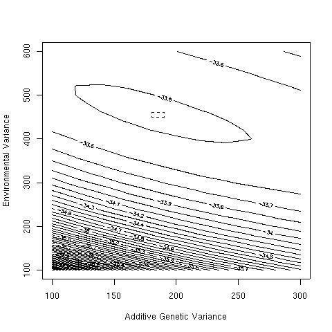
lik.surface(seq(100,300,20),seq(100,600,20))
points(maxlik$par[2], maxlik$par[3], pch=3)
rect(180,450,190,460,lty=2)
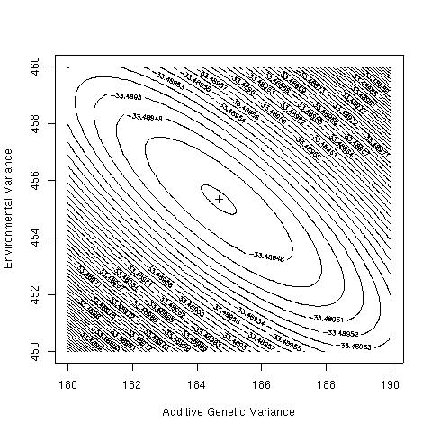
lik.surface(seq(180,190,0.1),seq(450,460,0.1))
points(maxlik$par[2], maxlik$par[3], pch=3)
|
The likelihood surface is smooth, and has its maximum of e-31.49 at VA=184.67 and VE=455.33. The heritability is therefore 29%.
|
|
|
Tambs et al [1992] collected systolic blood pressure measurements on 74994 Norwegians (88.1% of all residents in Nord-Trondelag county), and used census data to identify the various types of relative pairs present in the dataset:
| Relationship | Number of pairs | Correlation in sBP |
|---|---|---|
| R=1, K=1 | ||
| MZ twins | 79 | 0.521 |
| R=1/2, K=1/4 | ||
| Same-sex DZ twins | 90 | 0.154 |
| Brothers | 6017 | 0.220 |
| Sisters | 2856 | 0.211 |
| Brother-sister | 9278 | 0.193 |
| R=1/2, K=0 | ||
| Father-son | 10674 | 0.157 |
| Father-daughter | 8682 | 0.145 |
| Mother-son | 13262 | 0.165 |
| Mother-daughter | 10692 | 0.159 |
| Avuncular via MZ twins | 89 | 0.126 |
| R=1/4, K=0 | ||
| Grandparent-grandchild | 1251 | 0.065 |
| Avuncular via same-sex sibs | 598 | 0.140 |
| Avuncular via opposite-sex sibs | 548 | 0.083 |
| Cousins via MZ twins | 52 | 0.163 |
| R=1/8, K=0 | ||
| Cousins via same-sex sibs | 71 | -0.047 |
| Cousins via opposite-sex sibs | 17 | -0.172 |
| R=0, K=0 | ||
| Spouse | 23936 | 0.077 |
| Avuncular, spouse of same-sex sibs | 420 | -0.022 |
| Avuncular, spouse of opposite-sex sibs | 381 | 0.024 |
| Avuncular spouse of MZ twins | 66 | -0.110 |
We can make a semi-quantitative assessment of these correlations remembering the kinship coefficients for each type of relative pair.
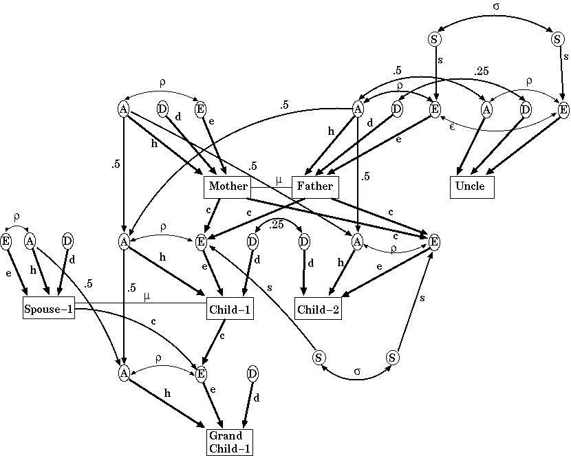
The model the authors used allowed for additive and dominance effects of polygenes, environmental effects shared by same-sex siblings, cultural transmission from parents to offspring, gene-environment correlation, and assortative mating. The equations predicting each correlation were derived from the following path diagram (Figure 2.2):
|
This looks quite formidable. The circles each represent the different causes of variation, A the additive genetic contribution of the polygenes; D the dominance genetic contributions; E all the environmental factors, S, those environmental components only shared by siblings of the same sex. The squares are the blood pressures for that type of individual. The lower case path coefficients are the regression coefficients to be estimated, and so represent the magnitude of the effects of the different variance components. For example, in the absence of assortative mating (so that mu=0), then h2 is equal to VA/VP in our earlier notation (since the trait variables have been standardised, VP=1).
By tracing each path from individual to individual one can write a simple equation for the correlations. For instance, the parent-offspring correlation is:
rpo = (1+u)(0.5 h (h + e p) + ec)
where,
u is the marital correlation in phenotype due to assortment,
h is the component of variation due to additive genetic contribution
of genes (correlated R between individuals),
e is the component of variation due to all environmental factors,
c is the cultural transmission from the parental phenotype to the
child's environment,
p is a correlation between the environmental and additive genetic
factors generated by the assortative mating and cultural transmission in the
parental generation's ancestors.
The model fitting was actually done using SAS (PROC NLIN), a standard statistical package, but had to ignore some complications as a result. For example, some individuals were counted twice, as they contributed both to the parent-offspring and sibling correlations. This will make the chi-squares used bigger (and standard errors smaller) than they should be, but will not affect the actual parameter estimates. It is possible to calculate a deflation factor (design effect) to allow for this problem.
The "best" model (chosen using the Akaike Information Criterion) included additive and dominance genetic components, a shared special same-sex sibling environment, assortative mating but no cultural parent to child transmission of blood pressure or gene-environment correlation. Under this model, VA=0.29, VD=0.18, and VE=0.53 (of which 0.02 is shared environment and 0.51 unshared environment).
A good example of complex segregation analysis is that of breast cancer in the Cancer and Steroid Hormone (CASH) Study [Newman et al 1988; Claus et al 1990; Claus et al 1991]. In that study, 4730 cases of early onset breast cancer (ages 20-54 years) presenting to eight centres from 1980-1982 were interviewed about the history of breast cancer in their mothers and sisters. In addition, 4688 age-region matched controls were also interviewed. A standard computer package (POINTER) allowed them to perform complex segregation analysis under the threshold model.
No family contained more than one proband, so the ascertainment was assumed to be single (that is, each entire family containing a breast cancer case has the same (small) probability of entering the study). In the preliminary case-control analyses (to geneticists, this would be known as a Weinberg proband-control analysis), it was shown that breast cancer risk to a family member increased with increasing strength of family history and decreasing age of diagnosis in the proband case:
| Family history | Hazard Ratio for breast cancer in sister of the proband case | ||
|---|---|---|---|
| proband onset 30 years | proband onset 40 years | proband onset 50 years | |
| No other affected first degree relative | 4.3 | 2.7 | 1.7 |
| An affected sister | 9.4 | 5.8 | 3.6 |
| An affected mother | 15.1 | 9.4 | 5.9 |
For the segregation analysis, Claus et al [1991] tested a two allele trait locus model with penetrances at seven age categories, and a residual family correlation due to polygenes. The best fitting model (in terms of model likelihood) was a high penetrance rare dominant locus (increasing allele frequency 0.0023) with no residual family correlation. By age 55 years, 46% of disease genotype carriers would have developed breast cancer, compared to 2% of those carrying the low risk genotype.
To further test the goodness of fit of the chosen model, Claus et al [1991] compared the predictions made by the model to the empirical recurrence risks to mothers and sisters from the case-control study. The segregation model predictions were fairly good for the families of the controls, and for sisters of probands, but did tend to underestimate the risk to mothers of a case, especially as the age at diagnosis of the proband increased.
Newman et al [1988] only analysed 1579 of the CASH families. They used the same computer program, but divided age into four classes. The best fitting model in this analysis was also dominant, with an allele frequency of 0.0006, and risk by age 55 of 66% in carriers. These authors also analysed a single large pedigree, which was also consistent with a highly penetrant dominant gene.
In the case of breast cancer, there are now two rare highly penetrant dominant loci that have been identified and cloned. In the Anglian Breast Cancer Study Group study [2000] of unselected breast cancer with age at diagnosis below 55 years, 0.7% were carrying a detectable BRCA1 mutation, and 1.3% a detectable BRCA2 mutation. The estimated frequency of such mutations in the general population was estimated at 0.0021 to 0.0031, and their penetrances at age 55 years at 30% (39% for BRCA1 and 25% for BRCA2). These are a little lower than those from the CASH study. By contrast, 2.2% of the Askenazi Jewish population in the US and elsewhere carry particular BRCA1 and BRCA2 mutations, with a similar penetrance at age 55. There are several relatively common loci that may also modify risk. One might expect the effects of such genes to appear in a segregation analysis as residual genetic correlation not explained by the major gene, but this is a function of how powerful the study is. Overall, one would conclude that the segregation analyses of breast cancer were fairly successful in determining whether genes of major effect were segregating in the population, and the frequency and penetrances of such genes.
In 1959, Abraham Lilienfeld performed a test of the robustness of the then available methods of classical segregation analysis. He showed that attending medical school was a phenotype that was strongly consistent with the action of a recessive gene. This analysis was updated by McGuffin and Huckle [1990], who presented data on family history in Welsh medical students. The segregation analysis program POINTER was used.
The sibling recurrence risk ratio for being a medical student was 100, and that for all first-degree relatives was 61. A model positing a SML with background additive polygenes ("mixed model") gave a significantly better fit than one assuming polygenes alone. Furthermore, a model assuming that only a SML was acting, fit just as well as the mixed model, with a recessive pattern of penetrances.
The gene for attending medical school therefore has a population frequency of 8.8%, and penetrances 0.346 and 0. The authors then continued to test the model assumptions by also estimating the transmission parameters. Merely estimating one transmission parameter (the 1/2 -> 1), as had been suggested in the literature did not allow them to reject the genetic hypothesis, but estimating all three parameters barely did (P=0.03).
This example demonstrates that results from segregation analyses need to be examined carefully and treated with caution. Many geneticists have little faith in complex segregation analysis, and would suggest moving straight from types of family study demonstrated in the first module to linkage analysis. However, the breast cancer example shows that the method can produce replicable, useful results, results that can be used to choose models for parametric linkage analysis.