Population genetics (and evolutionary genetics) deal with groups of organisms and families, usually natural populations. We can discern two strands of thought in the area. One is the study of very large ("ideal") idealised groups or populations, where models can be deterministic (though some deterministic models are accurate for even very small populations). The other is dealing with smaller populations, where the role of chance can play a larger role (so called genetic drift).
One question of crucial interest is this: how common are the different alleles at a given locus in a given population. In experimental plant and animal models, we obtained particular populations that were homozygous at a particular locus. For many genetically controlled traits of interest in natural populations, multiple alleles are segregating, more like the F2 generations in the experimental cross.
For a codominant trait, we can take a sample from the population, and count the different genotypes.
| Blood Group (genotype) | M (MM) | MN (MN) | N (NN) | Total |
|---|---|---|---|---|
| Count (percent) | 363 (28.4%) | 634 (49.6%) | 282 (22.0%) | 1279 (100.0%) |
The percentages are our best estimate of the probability that an individual will carry that genotype in the population of London, Oxford and Cambridge. The observed heterozygosity is 49.6%.
There is another population described in this table. It is the population of gametes that gave rise to individuals tested:
| Alleles | M | N | Total |
|---|---|---|---|
| Count (percent) | 1360 (53.2%) | 1198 (46.8%) | 2558 (100.0%) |
The percentages here are our best estimate of the probability that a sperm or egg taken from that population will carry that particular allele. If the frequency of the commonest allele at a particular locus is less than 99%, we call this a polymorphic locus or polymorphism.
Hardy-Weinberg equilibrium describes the relationship between the gametic or allele frequencies, and the resulting genotypic frequencies. It holds if the following properties are true for the given locus,
If these properties hold, then the probability that two gametes will meet and give rise to a new genotype is simply the product of the allele frequencies (a la binomial):
Pr(MM)= Pr(M) x Pr(M)
Pr(NN)= Pr(N) x Pr(N)
Pr(MN)= 1 - Pr(MM) - Pr(NN) = 2 x Pr(M) x Pr(N).
This can be also derived by enumerating all the possible mating types in the population, and using the Mendelian laws to derive the probabilities of the different offspring types. For the parental generation, let Pr(M)=p, Pr(N)=q, Pr(MM)=P, Pr(MN)=Q,Pr(NN)=R, p+q=1, P+Q+R=1:
| Mating | Proportion of Matings | Proportion of offspring | ||
|---|---|---|---|---|
| MM | MN | NN | ||
| MM x MM | P2 | P2 | -- | -- |
| MM x MN | 2PQ | PQ | PQ | -- |
| MM x NN | 2PR | -- | 2PR | -- |
| MN x MN | Q2 | Q2/4 | Q2/2 | Q2/4 |
| MN x NN | 2QR | -- | QR | QR |
| NN x NN | R2 | -- | -- | R2 |
| Total | (P+Q+R)2 | (P+Q/2)2 | 2(P+Q/2)(Q/2+R) | (Q/2+R)2 |
| 1 | p2 | 2pq | q2 | |
One can see that the assumptions of random mating etc affect the calculation of the mating probabilities in the second column. Furthermore, the HWE genotypic frequencies are attained in one generation, regardless of the distribution of genotype frequencies in the first generation.
We can easily test for deviation from Hardy-Weinberg equilibrium using a chi-square. This can arise from,
The first three effects will lead to fewer heterozygotes than expected under HWE. The effects of decreased viability depend on which genotype is deleterious.
Where dominance is present, we need to assume Hardy-Weinberg equilibrium to estimate allele frequencies. For a simple (fully penetrant) recessive (dichotomous) trait where the proportion of affected individuals in the population is R, the frequency of the increasing allele (ie increases probability or risk of being affected) will be R0.5. Then, the population frequency of the heterozygote will be 2(R0.5-R). For a dominant trait, the frequency of the increasing allele will be 1-(1-R)0.5.
Rather than quoting the observed heterozygosity for codominant multiallele markers (as we saw earlier for the blood group example), most workers in human genetics calculate the expected (or "average") heterozygosity (or gene diversity) based on the allele frequencies and assuming HWE. This is given by,
The gene diversity of a marker locus is, among other things, a measure of the utility of that marker for linkage analysis.
There are similar results for genotype and gametic frequencies at multiple loci. These are complicated if there is linkage between the loci. We will the examine the case of two loci.
In the parental generation, a locus A has two allelic forms A and a, with frequencies PA and 1-PA. A marker B has two alleles B and b (frequency PB). The recombination fraction between A and B is c. A parent can produce a gamete of either AB, Ab, aB, or ab.
The frequency of the different haplotypes in the gametes that gave rise to the parental generation are Pr(AB)=x1, Pr(Ab)=x2, Pr(aB)=x3 and Pr(ab)=x4. At equilibrium, the haplotype frequencies will be the product of the allele frequencies.
Linkage disequilibrium is expressed as the difference between this equilibrium value and that observed for the parental generation D=x1-PAPB. Another name for linkage disequilibrium is (intragametic) allelic association, where D is a measure of the strength of association between the alleles at the two loci eg the A and B alleles.
The gametic distribution emitted by all the parents in a population can be calculated by enumerating all the genotypes and then allowing for recombination events. For example, an AB gamete will be produced by a parent with the AB/AB genotype (population frequency x12) with probability 1, and by AB/ab genotype (coupling, population frequency 2x1x4) with probability (1-c)/2, and so on. Multiplying and summing probabilities we obtain,
| Gamete: | AB | Ab | aB | Ab |
|---|---|---|---|---|
| Frequency: | x1-Dc | x2+Dc | x3+Dc | x4-Dc |
so that D decreases each subsequent generation according to the recurrence relation [Jennings et al, 1917; Bennett 1954],
Therefore, if the two loci are unlinked, linkage disequilibrium will decrease by 50% in each generation. For loci separated by a recombination distance of 1%, a 50% decrease would take 69 generations. This is unlike the case for HWE, where equilibrium is reached after one generation.
By definition, D can take values from -PAPB to min[PA,PB]-PAPB. When comparing disequilibrium coefficients for different loci (or even for different alleles at the same multiallele locus), D is often rescaled, either by standardizing it to a binary correlation coefficient (dividing by its variance),
r=[PA(1-PA) PB(1-PB)]-0.5 D,
or expressing it as a proportion of its maximal value for the given allele frequencies (D').
D'=D/[min(PA,PB)-PAPB],
when D>0. Neither r (or r2) nor D' are completely satisfactory.
Many studies have attempted to survey the extent of linkage disequilibrium between loci in humans. Reich et al [2001] found D' in admixed-type European and US populations to average 0.95 between loci separated by 5 kb, 0.50 at 80 kb, and 0.35 at 160 kb (the average D' value for unlinked loci was 0.15).
In the case of a small (finite) population, where genetic drift is important, decay in disequilibrium per generation has been modelled as (Ohta and Kimura, 1968):
where Ne is the effective population size.
One of the mechanisms that can give rise to linkage disequilibrium is genetic mutation. This is the process by which new alleles at a locus appear, through mistakes in replication of a gene. As Maynard Smith [1989] states, "[i]f the replication process was exact, no new variants would arise, and evolution would slow down and stop."
Phenotypically, one will observe, in a homozygous line say, an offspring with a new phenotype that subsequently can be shown to obey Mendelian laws. For example, Schleger and Dickie [1971] present data for five loci controlling coat colour in mice. They detected 25 new mutations (deviations from the wild-type) in two million gametes tested (giving a probability of 1.1x10⁻⁵ per locus per generation).
In the case of dominant human diseases that have a marked effect on survival, and so reproductive success, mutation is the process leading to many or all new cases (depending on the severity of the disease). The mutation rates for these human loci are also approximately 10-5, ranging from 2x10⁻⁷ to 1x10⁻⁴, [see Vogel & Motulsky 1996]. For example, muation analysis of hemophilia B in the UK (with near complete ascertainment) gives rise to an estimate of 8x10⁻⁶ in males, and 2.2x10⁻⁶ in females [Green et al 1999].
Measuring divergence in protein-coding gene sequences between humans and other primates, Eyre-Walker & Keightley [1999] obtained similar rates, which they expressed as 4.2 coding mutations per genome (5x10⁴ genes) per generation, one-third of which are deleterious (novel or recurrent disease genes).
Rates have been measured directly for genetic markers in humans. Among the Simple Sequence Repeat markers, rates are proportional to heterozygosity [Weber & Wong 1993; Brinkmann et al 1998]:
| Heterozygosity | 50-65% | 70-75% | 90-99% |
|---|---|---|---|
| Observed mutations | 5.6x10⁻⁴ | 8.4x10⁻⁴ | 3.1x10⁻³ |
Kayser et al [2000] report an overall rate of 3.2x10⁻³ for 14 X-chromosome SSRs.
The nucleotide-wise mutation rate is understandably lower than the locus wise mutation rate: closer to 10-6. This is the generating mechanism for Single Nucleotide Polymorphisms (SNPs), and will randomly occur within coding or noncoding regions, approximately one per 1000 base pairs (derived as 1-(1-10-6)1000). Empirically in humans, the polymorphism rate is in fact around 0.8 per 1000 bp [eg Reich et al 2002]. Most human SNPs (99%) are monomorphic in chimpanzees [Hacia et al 1999; Stephens et al 2004], suggesting they have arisen over the 250000-300000 generations since divergence.
Deletion and insertion mutations are about 4 times less common than transversion SNPs (8% of all human polymorphisms) [Weber et al 2002]. The most common type is a single nucleotide deletion or insertion, but the length can be up to kilobases.
The repetitive nature of SSRs means it is easy for replication errors to occur. These are usually stepwise and limited in nature (an extension of a few repeats more than the original length). The different repeat lengths (alleles) at an SSRs are usually bimodal in distribution reflecting an original "big" step, followed by multiple "little" steps. This means it is often appropriate to combine alleles of similar length for studies of linkage disequilibrium.
SSRs occur within coding regions, where they can act as a "rheostat" controlling protein function that evolution can act on. The androgen receptor might be one model for this. Length-unstable coding triplet repeats are associated with several diseases, and in general coding SSRs are selected against.
More SSRs occur in the noncoding 5' and 3' untranslated regions flanking genes, and these may also be functional in modulating mRNA stability (DM1 and DM2 are possible examples), and acting as binding sites for nuclear proteins.
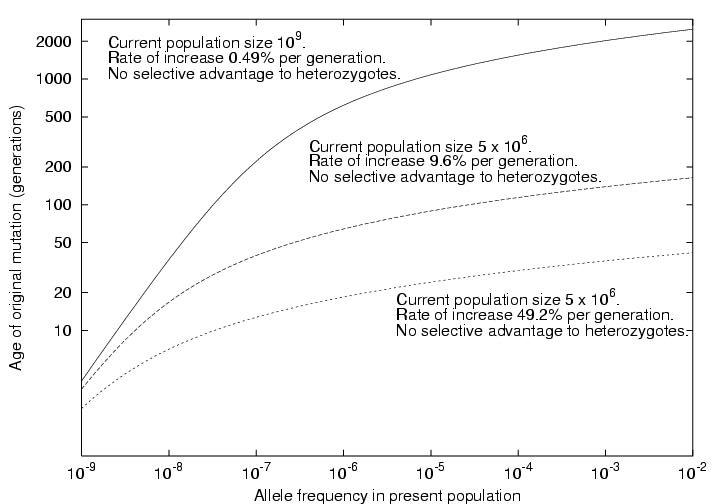
Slatkin and Rannala [1997] and Slatkin [2000] presented simple models for assessing the age of a mutant allele based solely on its population frequency. One model was based on linear birth-death processes, assume the mutant allele is not common, arose exactly once, but has not disappeared from the population. The second followed Griffith and Tavare [1998] in modelling the observed alleles as arisen from a coalescent process (a branching process followed backwards in time to the original mutational event). For a a neutral mutation (no effect on fitness or probability of leaving offspring of the carrier) in a population of constant size is linearly related to the number of generations (t) since the initial mutation event:
t*1 = 2 N p
where N is the population size, and p is the present allele frequency. This agrees well with the equation derived by Ohta [1973; Nei, 1975] under a different model again:
t = -{4Np/(1-p)} log(p)
In the case of an exponentially expanding population or one where the mutant allele is undergoing selection,
t*1 = log(2Np(r+s) + 1)/(r+s)
where r is the exponential growth rate parameter (approximately the proportional increase per generation), and s is the selection coefficient for heterozygotes. The equivalence between selection and exponential population growth is only approximate (see eg Slatkin [2001]). Values of r of 0.004 to 0.016 are plausible for older large populations (the world, or Western Europeans). For example, assuming N0=5000 founders t=2500 generations ago gave rise to to Nt=109 current descendents, substituting into:
Nt = N0 exp(rt)
gives r=0.0049. Hastabacka et al [1992] modelled r for the Finnish population as 0.09. This gives rise to the following relationship in such populations (assuming s=0):
A well-known example of such a calculation is for idiopathic torsion dystonia (locus DYT1) among the Ashkenazi Jews [Risch et al 1995]. In Eastern Europe, this population increased rapidly in size from approximately 105 in 1650 to 5 x 10⁶ in 1900, giving us an estimated r of 0.40. Risch et al [1995] estimate the allele frequency in the current population at 1/6000 to 1/2000. This gives an estimate of the age of the first mutation at 16-19 generations ago (about the year 1550).
If a new allele appears in a particular individual, and subsequently spreads through the population, alleles at loci closely linked to the mutated locus will be in linkage disequilibrium (associated) with the new allele. These alleles, those present in that first individual, make up an ancestral haplotype associated with the new trait. The length of this ancestral haplotype (in cM) is proportional to the age of the initial trait mutation.
Various models can be fitted to such data to estimate presence and strength of linkage disequilibrium, and mutation age.
The simplest model applies to two locus haplotypes. A marker locus B (alleles B and b with frequencies PB and 1-PB) is close to the trait locus A (recombination fraction c) and the trait mutation (A allele) occurred on a haplotype carrying the B allele marker. At this time, linkage disequilibrium is at its maximum value Dmax. After t generations it decays to its present value of D. Remembering our definition of D', we can reorganize the formula D(t)=(1-c)tD(0) as:
t = log(D')/log(1-c)
Risch et al [1995] perform a similar analysis. Instead of using D' as the measure of linkage disequilibrium, the results are derived in terms of Pexcess or delta [Bengtsson & Thomson 1981]. For this special case where PA =< PB, Pexcess=D'.
| PD | = Pr(B allele|A is other allele on haplotype) |
| = (PAPB+D)/PA = PB+D/PA | |
| Pexcess | = (PD-PB)/(1-PB) |
| = D/(PA(1-PB)) = D/Dmax |
Returning to the case of idiopathic torsion dystonia, the closest marker ASS is approximately 0.018 cM distant from DYT1, and Pexcess=(0.806-0.086)/(1-0.086)=0.788, and t*=13.1.
Varilo et al [1996] reverse this logic to estimate the recombination distance between variant late infantile neuronal ceroid lipofuscinosis (CLN5) and its nearest marker D13S162. Pexcess was 0.923 and pedigree analysis suggested the mutation to be 20-40 generations old. Based on this c was estimated at 0.002-0.004 (c*=1-exp(log(Pexcess)/t)).
Several authors have presented methods for detecting the effects of natural selection by comparing the estimated age based on allele frequency to that based on linkage disequilbrium [Slatkin 2000; Sabeti et al 2002; Toomajin et al 2003].
Finally, note that essentially the same equation is presented by Kaplan and Weir [1995], though with a different derivation. In their formula,
t = log(D')/(-c).
Those authors examine three methods for estimating an upper confidence bound on estimates of c or t. They concluded that one such estimator (the "Luria-Delbrook" moment estimator), suggested by Hastabacka et al [1992], gives a too small interval.
Genetic association studies take advantage of the fact that we can measure genotypes "directly". In classical terms, we are measuring a codominant trait, via protein electrophoretic or molecular genetic methods. In practice, we may sequence the actual genetic code and look for mutations at the nucleotide base level. We then choose another phenotype that interests us, such as presence or absence of a disease state, and attempt to detect a correlation between it and the measured genotype at the population or between-family level. That is, data for an association study has the form:
Phenotype <- Trait locus genotype <-D'-> Marker genotype ,
while for a linkage study it has the form:
P <-T<-c->M<-relationship->M<-c->T-> P
In the traits we have discussed to date, the relationship between the underlying genotype and the observed phenotype has been simple. These are often referred to as classical Mendelian, or simple Mendelian traits. In many traits of interest to human genetics, this relationship is more complex. For example, a genotype may give rise to a particular phenotype only in a proportion of individuals, and so must be described in a statistical manner. The probability that a particular phenotype P will be observed in a individual of genotype G, Pr(P|G), is the penetrance.
We will consider the case of a dichotomous trait (present or absent) under the control of a two allele locus (alleles A and a). We can then write a description of the trait in the population,
| Genotype | Frequency in Population (HWE) | Conditional probability, that an individual of that genotype is | |
|---|---|---|---|
| Affected | Unaffected | ||
| AA | PA2 | f2 | 1-f2 |
| Aa | 2PA(1-PA) | f1 | 1-f1 |
| aa | (1-PA)2 | f0 | 1-f0 |
Knowing the allele frequencies and penetrances, we can calculate the overall proportion of the population expressing the trait (affected),
Population Risk = PA2 f2 + 2PA(1-PA) f1 + (1-PA)2 f0.
This is a useful test to see if our model fits the data.
In the presence of covariates such as age or sex, the model is usually extended in a stratified fashion by defining liability classes, and defining penetrances for each liability class:
| Sex | PenAA | PenAB | PenBB |
|---|---|---|---|
| Male | f0m | f1m | f2m |
| Female | f0f | f1f | f2f |
A seminal (two page) paper by James [1971] demonstrates how to calculate concordances and recurrence risks for relatives under a specified SML. It is interesting because it applies linear modelling to probabilities. Let Prob be a random binary variable representing disease status in an individual and Rel be a similar variable for a relative of our proband:
| Pr(Prob=1,Rel=1)= | Cov(Prob,Rel) + Prev2 |
| Pr(Prob=1|Rel=1)= | Prev + Cov(Prob,Rel)/Prev |
| Cov(Prob,Rel)= | R.VA + K.VD |
| VA= | 2PA(1-PA)[ PA(f2-f1) + (1-PA)(f1-f0)]2 |
| VD= | P2A(1-PA)2 [f2-2f1+f0]2 |
R and K are the coefficients of relationship and fraternity respectively. The coefficient of relationship is the probability that one allele at a locus in the proband is the same as that in the relative by descent, and the coefficient of fraternity is the probability both are identical by descent.
| Type of Relative Pair | R | K |
| Monozygotic Twins | 1 | 1 |
| Siblings/Dizygotic Twins | 1/2 | 1/4 |
| Half-Siblings | 1/4 | 0 |
| Parent-Offspring | 1/2 | 0 |
| Unilineal kth degree relative pair | 1/2k | 0 |
| Uncle-Nephew | 1/4 | 0 |
| Cousins | 1/8 | 0 |
The frequency of the APOE*4 allele of the APOE locus is approximately 15% in Caucasian populations. In one study of Finns aged 69-78 years, the authors observed,
| Genotype | Number (percent) diagnosed with Alzheimers | Total number with genotype |
|---|---|---|
| E4/E4 | 6 (21.4%) | 28 |
| E4/+ | 21 (7.6%) | 277 |
| +/+ | 19 (2.9%) | 652 |
| Total | 46 (4.7%) | 957 |
The frequency of the E4 allele in the sample is 17.4%, and the genotype frequencies are not significantly different from HWE (X21=0.05). The penetrances differ markedly from one another (X22=26.7, P=1x10⁻⁶). The estimated penetrances are roughly multiplicative (increasing about 2.5 fold with each additional E*4 allele). The cumulative risk of AD to age 75 (approximately) in the whole sample is 4.7%, close to that from other population studies of AD.
Cordell et al [1993] report a similar study that looked at a sample of 234 individuals where all had a family history of AD. They report penetrances (at age 75) of f2=86%, f1=61%, and f0=24%. If we use an E*4 allele frequency of 15%, these penetrance figures predict a population risk of,
0.152 x (0.86) + 2 x 0.15 x 0.85 x (0.61) + 0.852 x (0.24) = 35%.
This is much higher than the overall population risk, and suggests that their sample of subjects was different from the general population (probably because they were carrying other AD genes).
The AD studies were cross-sectional in nature, that is we examined a simple sample from a particular population. The more common approach to this type of study is a case-control approach. In a case-control study we collect two samples, one containing affected individuals, the second containing unaffected individuals. We can calculate a chi-square for the homogeneity of the allele or genotype frequencies between the two groups. We do not get a simple estimate of the penetrances or allele frequencies, as in the case of the cross-sectional study, but we will probably have to genotype fewer subjects to get the same size chi-square.
It is possible to calculate penetrances from a case-control study, providing we have some additional information: the allele frequencies and the overall population risk. If the trait is sufficiently rare, then the allele frequencies in the control group will be similar to those in the general population, and we can use these as an estimate of the population allele frequencies.
Since the proportion of the population affected is,
R = PA2 f2 + 2PA(1-PA) f1 + (1-PA)2 f0,
then the proportion of individuals within that affected group with the different genotypes will be,
| Genotype | AA | Aa | aa |
|---|---|---|---|
| Probability | PA2f2/R | 2PA(1-PA)f1/R | (1-PA)2f0/R |
If we are unable to obtain an estimate of the population risk R from another source, we will have to be content with an estimate of the ratios of the penetrances to one another.
Here is a case-control study of 91 consecutive AD patients at a Montreal referral centre who were compared to a control group made up of healthy spouses and "elderly volunteers".
| Group | Genotype Count (Percent) | |||
|---|---|---|---|---|
| E4/E4 | E4/+ | +/+ | Total | |
| Alzheimer's Disease patients | 12 (13%) | 46 (50%) | 33 (36%) | 91 |
| Unaffected controls | 2 (3%) | 14 (19%) | 55 (79%) | 71 |
The chi-square comparing genotype frequencies is just as large as that obtained in the Finnish study (X22=27.7), which suggests that there are significant differences in the penetrances of the APOE genotypes.
If we take the APOE*4 allele frequency as 15%, and the population risk at 5%, then the estimated penetrances are f2=0.29, f1=0.10, f0=0.025, which are in reasonable agreement with the Finnish data.
Instead of comparing genotype frequencies, it is often more powerful to compare allele frequencies in the two groups. If we do that in this case we obtain,
| Group | Allele counts (percent) | ||
|---|---|---|---|
| E4 | + | Total | |
| AD patients | 70 (38.5%) | 112 | 182 |
| Controls | 18 (12.7%) | 124 | 142 |
The chi-square testing the difference in proportions gives X21=26.81, with a P=2.2x10⁻⁷. In other words, we obtained roughly the same chi-square value, but now we only have one degree of freedom. The reason this allelic test is more powerful is that it has a simpler alternative hypothesis. It assumes that the pattern of penetrances is multiplicative, that is that f2/f1 is equal to f1/f0, and that HWE holds (in the base population). Usually, a test designed to test a specific alternative hypothesis is more powerful than a more general test if the alternative hypothesis is (roughly) correct. If the heterozygotes had a higher risk of AD than either of the homozygotes, this test would be less powerful than the genotypic test. In practice, heterosis (f1>f0 and f1>f2) is not common. If HWE does not hold, it is still possible to fit a multiplicative penetrance model as a Berry-Armitage trend test or logistic regression.
If we assume that 5% of the population this age have AD, then these data would predict a population E4 allele frequency of 0.05*(0.385)+0.95*(0.127)=14%, which is pretty close to the 15% we have been working with. Using the 12.7% in the controls as an estimate for our penetrance calculations wouldn't make a large difference.
Using the results of James [1971], we can test whether APOE is sufficient to explain all the familial aggregation of AD, excluding the rare early-onset types. Martinez et al [1998] examined the recurrence risk of AD in first degree relatives of 290 late-onset AD probands.
The crude recurrence risk was 11.7%. If we take the baseline risk to be 5%, then the recurrence risk ratio is 2.3. Under the pattern of penetrances estimated in the Finnish study for APOE, the expected RRR is only 1.25. The patterns replicate those mentioned earlier from Cordell et al [1993].
The estimated lifetime penetrances in these relatives were actually:
| Genotype | Penetrance | |
|---|---|---|
| Genotype | Martinez et al [2000] | Kuusisto et al [1994] |
| APOE*3/*3 | 0.292 | 0.029 |
| APOE*3/*4 | 0.461 | 0.076 |
| APOE*4/*4 | 0.614 | 0.214 |
In non-genetic situations in epidemiology, the favourite measure of association in a case- control study is the odds ratio. Take a genotypic table of counts from a case-control study,
| Group | Genotype Count | ||
|---|---|---|---|
| AA | Aa | aa | |
| Cases | a | b | c |
| Controls | d | e | f |
There are three sets of odds. The odds of being a case, given the genotype AA are a/d, for Aa they are b/e, and for aa, they are c/f. These odds can be compared to one another. So the odds ratio comparing Aa to aa is,
OR10 = (b/e) / (c/f) = bf/ce,
and that comparing AA to aa is,
OR20 = (a/d) / (c/f) = af/cd.
If there is no effect of genotype on risk of disease, then OR10=OR20=1. It is easy to calculate confidence intervals for odds ratios. If the trait is rare in the general population, it can be shown that the odds ratio is approximately equal to the risk ratio (or relative risk),
OR10 = f1/f0, and OR20 = f2/f0.
If a multiplicative model for the penetrances is correct, then the allelic table,
| Group | Allele Count | |
|---|---|---|
| A | a | |
| Cases | a | b |
| Controls | c | d |
gives an odds ratio,
OR=ad/bc,
that summarizes the ratios of the penetrances, and thus increase in risk to carriers of one or two increasing alleles compared to those carrying none (the decreasing homozygote).
There are two ways to interpret the results of genetic association studies. In the first approach, we take ApoE as being the genotype, and AD the phenotype. We then attempt to estimate the penetrances. This assumes that the genotype, is causing the phenotype AD.
In the second interpretation, we take two genetics traits -- the codominant ApoE trait, and the AD trait, for which we have no good genetic model (but know that it aggregates within families), and try to detect allelic association or linkage disequilibrium. The "penetrances" that we estimate are then a mixture of the effects of the AD gene, and the strength of the linkage disequilibrium between the two loci. We have no way of differentiating between these two hypotheses, because we don't know what the AD genotypes are.
We can get around the problem just alluded to by examining multiple tightly linked marker loci. This approach to fine mapping is seeing extensive development at the moment. At its simplest level, it is multiple separate case-control analyses, but more elaborate multilocus models are based on coalescent processes for example.
For a haplotype spanning such a set of markers, the probability that two chromosomes taken from the population will be identical by descent is 1/(1+4 Nec-2c-2 Nec2+c2) [Sved & Feldman 1973].
Martin et al [2000] attempted to exclude genes close to APOE as the true AD locus. There were 220 cases and 220 controls genotyped at 60 SNP markers.

The authors have chosen the chi-square P-value as their test statistic. There are several notches among the peak values. Some of these are due to that marker having low heterozygosity (one allele is relatively rare).
Another mechanism is historical. If a single mutation event lead to the creation of the APOE*3 allele, with its reduction in risk of AD, then if the neighbouring marker allele on that ancestral haplotype was common, the frequencies of that allele in cases and controls will be similar. If the marker allele was previously generally rare, then as APOE*3 became more common in the population, "hitchhiking" causes the case-control difference in marker allele frequencies to become easier to detect.
The method of antigen genotype frequencies among patients (Bodmer & Bodmer 1974; Thomson 1983) uses counts of the different genotypes in affected individuals only. It assumes that the genotype that we have measured is not at the trait locus, but is in linkage disequilibrium with it. It further assumes that the trait locus has a simple mode of inheritance, such as autosomal dominant or recessive, and attempts to test which pattern of penetrances best fits the data.
For a recessive trait locus (f2>0, f1=f0=0), the expected values for the three genotypes in the sample of affected individuals are simply the HWE expectations, where the marker allele frequency is that based on the cases. For a uncommon dominant (f2=f1>0, f0=0) or additive (f2-f1=f1>0, f0=0), the "allele frequency" used is twice the allele frequency in the cases minus the allele frequency in the general population (or controls). These tests are generally not very powerful, but in simple Mendelian traits, can be useful.
| 27/27 | 27/+ | +/+ | X2 | |
|---|---|---|---|---|
| Observed Count | 3 | 70 | 6 | -- |
| Recessive Hypothesis | 18.3 | 39.4 | 21.3 | 47.55 |
| Additive Hypothesis | 3.4 | 69.1 | 6.5 | 0.097 |
Here the recessive hypothesis does not fit the data at all well. The additive hypothesis, by contrast, gives expected counts very close to those observed. If we apply the same method to the AD case-control data, we get a recessive X21=0.42, and an additive X21=2.53. We can't draw any firm conclusions.
Several authors have applied a related approach as a tool for fine mapping, most successfully to detect the hemochromatosis gene HFE [Feder et al 1996; Thomas et al 1999].
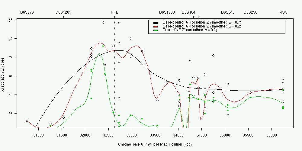
In this case, the Hardy-Weinberg equilibrium test was applied to 101 cases (AGFAP test for the recessive model). In the plot (data from Thomas et al 1999), the green points and line are the results for each marker and a smoothed multipoint curve. The open circles are the results from the equivalent case-control analysis (adding 61 controls).
The peak HWE X2 was 112.3 for a C282Y polymorphism in the HFE gene (not shown in the plot, Z=10.6). This argues against the simple autosomal recessive AGFAP model that the penetrance of the C282/C282 and C282/Y282 genotypes is zero (though the dominant model is even more strongly rejected, X2=2025). It also highlights why other authors have had less success using this for fine mapping. Here are results from Martin et al [2000] again:

We collect data for two diallelic codominant loci (A and B) from a population sample. We have not collected family information, so we are unable to determine the phase of the genotypes (coupling or repulsion).
| AA | Aa | aa | Total | |
|---|---|---|---|---|
| BB | n22 | n21 | n20 | NBB |
| Bb | n12 | n11 | n10 | NBb |
| bb | n02 | n01 | n00 | Nbb |
| Total | NAA | NAa | Naa | NT |
Under complete (Hardy-Weinberg and linkage) equilibrium, the expected proportions are easy to calculate. For example, n22=PA2PB2, where PA is the frequency of the A allele, (2NAA+NAa)/2NT. This can be used to construct a chi-square test for this composite null hypothesis.
We can partition out this full chi-square into four components. Two are due to deviation from HWE at each locus. The third measures the level of allelic association or linkage disequilibrium. However, this table describes genotypes and not haplotypes, so there is a remaining component that measures intergametic association. This is due to correlations in the parental genotypes that might arise from population stratification, for example, and so is more akin to Hardy-Weinberg disequilibrium than linkage equilibrium. For example, like H-W disequilibrium, it dissipates quickly following the introduction of panmixia.
The expected values, if HWE holds, allelic association is present, and intergametic association is absent, are,
| AA | Aa | aa | |
|---|---|---|---|
| BB | x12 | 2x1x3 | x32 |
| Bb | 2x1x2 | 2(x1x4+x2x3) | 2x3x4 |
| bb | x22 | 2x2x4 | x42 |
Here,
| x1=PAPB+D, |
| x2=PA(1-PB)-D, |
| x3=(1-PA)PB-D, |
| x4=(1-PA)(1-PB)+D. |
The remaining chi-square for intergametic disequilibria is calculated by subtracting the other three chi-squares from the total. The actual calculation of the expected counts and chi-square statistics is complex, and is best left to a computer program, which can also give an estimate of the size of D.
Most of these association analyses can be carried out using standard statistical packages such as SAS, SPSS, GLIM, or BDMP. There are a number of free packages that are suitable:
For these problems, you will need the Linkage utility programs.
(1a) Moffat and Cookson (1996) performed a study of 92 subjects with asthma, and 318 nonasthmatics from Busselton, West Australia. They typed these subjects at two closely linked markers, LTA (coding for tumour necrosis factor alpha) and TNF (tumour necrosis factor beta), on chromosome 6:
| 1,1 | 1,2 | 2,2 | |||
|---|---|---|---|---|---|
| LTA NcoI | Asthma | No | 35 | 137 | 141 |
| Yes | 19 | 42 | 27 | ||
| TNF-308 | Asthma | No | 211 | 89 | 12 |
| Yes | 44 | 36 | 8 |
Is there allelic association between either of these loci and asthma?
(1b) Shimura (1994) and Badenhoop (1992) give frequencies for the LTA NcoI polymorphism in two control samples:
| 1,1 | 1,2 | 2,2 | |
|---|---|---|---|
| Shimura (Japan) | 21 | 56 | 88 |
| Badenhoop (Europe) | 17 | 72 | 84 |
Are these in HWE? Can they be combined to give a pooled estimate of the frequency of this polymorphism? How do they compare to the frequencies in the control group from the Busselton sample?
(1c) If you were told that the frequency of asthma in the Busselton population is 9%, what would the "penetrances" of LTA for asthma be? Why did I put "penetrances" in quotes?
(1d) Shimura also genotyped lung cancer patients at the LTA locus, and obtained N11=27, N22=52, N12=56. Is there evidence for an association here?
(1e) Badenhoop performed a similar analysis for individuals suffering from Graves disease. He obtained,
| 1,1 | 1,2 | 2,2 |
|---|---|---|
| 18 | 96 | 60 |
Is LTA also associated with Grave's Disease?
(2) Thomson gives the following for the distribution of the HLA-A3 allele in a sample of patients with hemochromatosis:
Number with "A3/A3" genotype, 20; "A3/-" genotype, 43; "-/-" genotype, 21. Furthermore, the population frequency of the A3 allele is 0.146. Based on this information, is there allelic association between HLA-A and hemochromatosis? What simple Mendelian model best fits the data?
(3) Mourant (1976) typed 537 individuals at the MN and S blood groups. These loci are known to be tightly linked. He obtained the following results:
| SS | Ss | ss | |
|---|---|---|---|
| MM | 91 | 147 | 85 |
| MN | 32 | 78 | 75 |
| NN | 5 | 17 | 7 |
Test for the various types of equilibrium. What conclusions do you draw?
In order to give valid results, the population-based and case-control association studies described above require certain properties to hold. Most critically, they require random mating in the population. If population stratification is present or has occurred in the recent past, then this can give rise to association between alleles that is not due to linkage disequilibrium between loci on the same chromosome. To take a trivial example (after Lander), say ethnic Chinese carry an allele not found in other groups (a private polymorphism). Then, a case-control study that includes a mixture of subjects of different ethnicity (creating an artificial stratified population) will conclude that a gene for ability to use chopsticks is in linkage disequilibrium with the private polymorphism.
Knowler et al (1988) give a slightly more subtle real-life example. The Pima Indians of Arizona have high rates of non-insulin-dependent diabetes mellitus (NIDDM), and have been intensively studied by geneticists. In a sample of 4920 subjects from Gila River Indian Community,
| Genotype | Number (percent) diagnosed NIDDM | Total number with genotype |
|---|---|---|
| G/G or G/+ | 23 (8%) | 293 |
| +/+ | 1343 (29%) | 4627 |
| Total | 1366 (28%) | 4920 |
This shows a strong association between the "wild type" haplotype(s) and being diabetic. However, the authors were aware of the fact that the Gm3;5,13,14 haplotype was less common in "full-blood" Pimas,
| Haplotype | Indian heritage | ||||||
|---|---|---|---|---|---|---|---|
| 0/8 | 1/4 | 3/8 | 1/2 | 3/4 | 7/8 | Full | |
| G | 28 (43%) | 20 (56%) | 4 (9%) | 146 (21%) | 27 (14%) | 13 (5%) | 70 (1%) |
| + | 36 | 16 | 42 | 542 | 171 | 259 | 8458 |
Our suspicions should also be aroused by a large excess of heterozygotes in the sample (marked violation of HWE). When the authors performed a stratified analysis of NIDDM, they instead found,
| Half-Pima | Full-Pima | |||
|---|---|---|---|---|
| Genotype | Number (percent) NIDDM | Total number with genotype | Number (percent) NIDDM | Total number with genotype |
| G/G or G/+ | 5 (18%) | 28 | 12 (40%) | 30 |
| +/+ | 7 (26%) | 27 | 1242 (49%) | 2514 |
| Total | 12 (22%) | 55 | 1254 (49%) | 2544 |
This shows that the higher the Indian heritage, the greater the risk of NIDDM (as expected). Within each stratum or subpopulation, there is no significant difference in the rates of NIDDM for the different genotypes. It is possible to calculate a homogeneity chi-square comparing the within-stratum differences across each level of Indian heritage and of age. This showed that the results from each stratum are consistent in showing no effect of Gm haplotype once ethnicity is allowed for.
Therefore, there is linkage disequilibrium, but it has been generated by recent population admixture. Any locus with different allele frequencies in the original Caucasian and Pima populations will exhibit disequilibrium with the Pima NIDDM susceptibility locus, regardless of their chromosomal locations. We will have to wait several generations of random mating for the disequilibrium between unlinked loci to wash out, leaving only the "interesting" associations between alleles at loci with r<<50%.
Another example was presented by Hirschhorn et al [2004]. These authors describe a study comparing gene frequencies in individuals from the 5-10th percentiles (N=176) and 90-95th percentiles (N=192) of height. Over 100 diallelic polymorphisms were genotyped. Comparison of allele frequencies in the two groups was not suggestive of admixture. However when genotype at the -13910C>T lactase persistance polymorphism was tested for association using a larger panel (N=2288), this showed strong evidence of association. Allele frequencies at this polymorphism vary greatly from Northern to Southern Europe, and stratifying on ancestry greatly reduced the strength of association.
For a case-control design, these effects are dealt with by appropriate ethnic matching of the control group with the case group. Therefore, we select controls to fill up the one or more strata, so that we are testing (hopefully) within the same randomly mating populations.
Falk and Rubinstein (1987) suggested the best place to get an ethnically matched control for a case-control study is in the family of the case. One way to do this might be to use an unaffected sibling as a control. Their suggestion was use the parents. Because each parent contributes one allele to the case, the control allele must be the allele not transmitted to the affected child. So, if the parents are genotypes A/a and a/a, and the child is a/a, the case has genotype a/a, and the "control" has genotype A/a. These counts are analysed as if they came from a conventional case-control study.
Ascertainment is the term geneticists use for sampling. I have mentioned two types of sampling so far. In the case of the cross-sectional population samples, these were simple samples -- either a complete sample, or a simple random sample. This meant that the allele and trait frequencies in the sample reproduced the frequencies in the total population. The case-control design uses a stratified sampling, where we collect particular numbers of individuals with different trait values. This means that the frequency of the different trait types in the study is fixed by the design, and not by the population frequencies.
In genetics, more complex ascertainment schemes are often used. For a start, these often involve families rather than individuals (as in the HRR example). Fixing on nuclear families, under "complete" ascertainment, or truncate selection, we select all, or a simple random sample of, the nuclear families where at least one child expresses a particular binary trait. Or we might select families where at least one parent is affected, or where at least two children are affected. An individual that leads to a family being included in the sample is called a proband or propositus.
If the population being sampled, and the sampling rule, can be adequately described, we can work out the probabilities involved. These allow us to calculate expected values for a chi-square or other analysis.
In many cases, for an ascertained sample, the expected values under the null hypothesis of no linkage or no allelic association are simply those for the total population. That is, if the trait that the sample has been ascertained upon is unrelated to the marker locus, then allele or genotype frequencies will be unchanged, as will the Mendelian segregation ratios. In the case-control study for example, under the null hypothesis, the genotype frequencies in the ascertained case group will be the same as in the control group.
If one has genotyped an affected child and the parents, an alternative approach to a case-control HRR analysis is to test for deviations from the Mendelian ratios. Under the null hypothesis of no effect of ascertainment on segregation, Flanders and Khouri (1996) suggest a four degree-of-freedom chi-square of this familiar table (diallelic marker locus),
| Mating Type | Number of matings | Observed genotype counts in proband | Expected genotype counts in proband | ||||
|---|---|---|---|---|---|---|---|
| AA | Aa | aa | AA | Aa | aa | ||
| AA x Aa | N1 | O1 | O2 | -- | N1/2 | N1/2 | -- |
| Aa x Aa | N2 | O3 | O4 | O5 | N2/4 | N2/2 | N2/4 |
| Aa x aa | N3 | -- | O6 | O7 | -- | N3/2 | N3/2 |
Note that only the matings where different genotypes are segregating in the offspring are useful. Furthermore, the authors suggest how to calculate the ratios of the penetrances using this table, as we can for a case-control study, using the ratios of observed to expected counts:
f1/f0= (O4/E4+O6/E6) / (O5/E5+O7/E7),
and,
f2/f0=(O3/E3) / (O5/E5).
We can break up this contingency table even further. The only time we get informative offspring is when one or both of the parents is heterozygous. In the matings where only one parent is heterozygous, all the information is coming from that parent. If we assume random mating (this is slightly simplified), we can create a simpler table looking at alleles rather than genotypes,
| Parental Genotype | Number of such Parents | Observed Counts | Expected Counts | ||
|---|---|---|---|---|---|
| A | a | A | a | ||
| Aa | N | O1 | O2 | N | N |
Here N=N1+2N2+N3 from the earlier table. This leaves us with a binomial test comparing the observed ratio O1/N with its expectation of 50%. This test is what Spielman et al (1992) called the transmission-disequilibrium test (TDT).
| AB | Ab | aB | ab | |
|---|---|---|---|---|
| AB | f2(x1-Dc)2/R | f2(x1-Dc)(x2+Dc)/R | f1(x1-Dc)(x3+Dc)/R | f1((x1-Dc)(x4-Dc)/R |
| Ab | f2(x1-Dc)(x2+Dc)/R | f2(x2+Dc)2/R | f1(x2+Dc)(x3+Dc)/R | f1(x2+Dc)(x4-Dc)/R |
| aB | f1(x1-Dc)(x3+Dc)/R | f1(x2+Dc)(x3+Dc)/R | f0(x3+Dc)2/R | f0(x3+Dc)(x4- Dc)/R |
| ab | f1(x1-Dc)(x4-Dc)/R | f1(x2+Dc)(x4-Dc)/R | f0(x3+Dc)(x4-Dc)/R | f0(x4-Dc)2/R |
where, as before,
R=P(trait expressed)=PA2f2+2PA(1-PA)f1+(1-PA)2f0.
The probability that the proband receives a trait allele from a parent is:
P(Receive A)= t(A) = PA[(f2-f1)PA+f1]/R
P(Receive a)= t(a) = 1-t(A) = (1-PA)[(f1-f0)PA+f0]/R
For example, if A acts as an autosomal recessive, f2=f, f1=f0=0, then t(A)=1. For an autosomal dominant, f2=f1=f, f0=0, t(A)=1/(2-PA).
Denoting the rows of the table above as the transmitted haplotype, and columns as nontransmitted haplotypes, we can further condition on the probability of transmission (multiplying the top two rows by t(A)/PA, and bottom two rows by t(a)/(1-PA), and then collapse over the (unobserved) A genotypes, and write t(A)/PA-t(a)/(1-PA) as T,
| Nontranmitted | ||||
|---|---|---|---|---|
| B | b | |||
| Transmitted | B | PB2+PBTD | (1-PB)PB+(1-PB)TD - TDc | PB+TD(1-c) |
| b | (1-PB)PB-PBTD + TDc | (1-PB)2-(1-PB)TD | (1-PB)-TD(1-c) | |
| PB+TDc | (1-PB)-TDc | 1 | ||
We have already decided that the only useful parents are heterozygous, so the two counts contributing to the TDT are: B transmitted, b not transmitted; and b transmitted, B not transmitted. The expression for the expected ratio for the TDT is complex. If we take the difference between the expected counts (B or b transmitted), we get a simple expression,
Difference = TD(1-2c)
Therefore, the TDT is testing the joint null hypothesis: c=0.5 or D=0. Warren Ewens, at GAW9, described the TDT as a test for linkage, in that the disequilibrium D can actually be due to population admixture. Nevertheless, it has the advantage of being most powerful when the allelic association has arisen between tightly linked markers, thus giving us a chromosomal location for the trait locus.
The one degree-of-freedom chi-square (approximating the binomial test when counts are sufficiently large) is:
T is seen to be more crucial than t(A), and reduces to:
The first term of the numerator is a dominance term, so the TDT lacks power when the trait gene acts in an additive fashion. Again, for an autosomal dominant, T=(1- PA)/PA(2-PA), and for a recessive, 1/PA.
I have limited the discussion to date to the two allele case. In practice, we may be using a microsatellite marker or a SNP haplotype, so there will be many alleles. Extending the TDT to the case of a multiallelic marker locus is straightforward. We will limit ourselves to A having two alleles as before (now denoted A1 and A2), but B now has m alleles (B1...Bm), each of which may exhibit different levels of association with the trait locus alleles, Dij, for Bi, Bj, i=1..m-1, j=i..m. One mechanism by which this model could arise would be recurrent mutation at A of A2A1, so that in the absence of forces opposing linkage equilibrium, the degree of allelic association for different alleles of A and B will reflect different ages of the A mutation.
The properties of the disequilibrium measure used here need slight amplification. If B has 3 alleles, there are 3 covariances (one of which is a function of the other two):
D12=P(A1B1).P(A2B2)-P(A2B1).P(A1B2);
D13=P(A1B1).P(A2B3)-P(A2B1).P(A1B3);
D23=P(A1B2).P(A2B3)-P(A2B2).P(A1B3).
The haplotype frequencies can still be written in terms of allelic frequencies and disequilibria: P(A1B1)=[P(A1)P(B1)- D12]/[P(B1)+P(B2)] etc.
It can be seen that the choice of model and measure of covariance allows direct extension of our earlier results. The parental gametic output array now contains elements,
P(AiBk|AiBl)=P(AiBk).P(AiBl), i=1..2, k=1..m, l=1..m
P(AiBk|AjBk)=P(AiBk).P(AjBk), i ne j
P(AiBk|AjBl)=P(AiBk).P(AjBl)+rDkl, i ne j, k<l
P(AiBk|AjBl)=P(AiBk).P(AjBl)-rDkl, i ne j, k>l.
The matched transmission-nontransmission table conditioned on the proband has off-diagonal entries:
Pr(Tr=Bk, NT=Bl)= P(Bl)/[P(Bk)+P(Bl)] . (P(Bk)+TDkl)-TDklc
where Tr and NT are the transmitted and nontransmitted alleles respectively.
A global test procedure for such a square table where the null hypothesis is that of symmetry, that is, Pkl=Plk for k=1..m, l=1..m, l ne k, are the goodness-of-fit statistics:
This turns out to be equivalent to performing a one degree of freedom TDT for each type of heterozygous parent, and adding up the resulting chi-squares. This test is what Sham and Curtis called the "genotypic" TDT, but what I prefer to call an omnibus or global allelic TDT.
Alternative tests compare the marginal totals of transmitted and nontransmitted alleles. These are either maximum likelihood based (constructed by subtracting a "quasi-symmetry" chi-square term from the full symmetry chi-square described above) or a score test (Stuart's Q statistic). These are probably slightly more powerful than the full symmetry test.
For completeness, I'll return to the genotypic HRR tests for a diallelic marker. Knapp et al (1993) showed the marker genotype frequencies among the affected offspring are,
| BB | PB2 | + 2PBA + B - 2cPBA - 2cB + c2 B |
|---|---|---|
| Bb | 2PB(1-PB) | + 2(1-2PB)A - 2B- 22c(1-2PB)A + 4cB - 2cB |
| bb | (1-PB)2 | + 2(1-PB)A + B + 2c(1-PB)A - 2cB + c2B |
and the nontransmitted genotypes (combining the nontransmitted alleles),
| BB | PB2 | + 2cPBA + c2 B |
|---|---|---|
| Bb | 2PB(1-PB) | + 2c(1-2PB)A - 2c2B |
| bb | (1-PB)2 | - 2c(1-PB)A + c2B |
where,
A=D [PA(f0-f1)+(1-PA)(f1-f2)]/R,
and,
B=D2 [(f0-f1)+(f1-f2)]/R.
Therefore, if c=0, the nontransmitted genotype frequencies will be an estimate for the population frequencies. If c is greater than zero, then the genotype frequencies will be biassed away from the true values. Also, the odds ratios calculated from the HRR table (as if it were a conventional case-control study) will be biassed downwards, and the confidence intervals around these odds ratios will be too large.
For a genotypic TDT, there are similar expressions. The chi-square for testing these will still be a test of the counts nkl=nlk,
| Nontransmitted | ||||
|---|---|---|---|---|
| BB | Bb | bb | ||
| Transmitted | BB | n11 | n12 | n13 |
| Bb | n21 | n22 | n23 | |
| bb | n31 | n32 | n33 | |
Schaid and several others have pointed out a genotypic TDT can be formulated as a "pseudo-control" matched case-control study. The controls are the four genotypes a mating can give rise to, and the case is the observed case genotype. Standard statistical software can be used to fit this model. This allows the easy incorporation of covariates -- though the regression coefficients represent the interaction between gene and covariate.
I'll briefly discuss a couple more tests. What if the control is an unaffected sib rather than the nontransmitted parental alleles. The table will look like this (where parental genotypes are available),
| Heterozygous parent tranmsitted | ||
|---|---|---|
| A | a | |
| Affected Child | O1 | O2 |
| Unaffected Child | O3 | O4 |
Again, there is no "within-family" information if the parents are homozygous. One approach is to compare transmission to the affected and unaffected children, that is do an independence chi-square. This seems a little stupid, when we recall that we know that the segregation ratios must be 50% in each group under the null. The best approach then will be to do two TDTs, one for each group, and combine the results. Unless the trait is particularly common, the "unaffected" TDT will not be very powerful. Another might be to take the sibship as the unit of analysis,
| Sibship type, Aa x AA mating | Frequency of each sibship type | ||
|---|---|---|---|
| Affected received | Unaffected received | Observed | Expected under null hypothesis |
| AA | AA | O1 | N/4 |
| AA | aA | O2 | N/4 |
| aA | AA | O3 | N/4 |
| aA | aA | O4 | N/4 |
| Total Number of Sibships | N | N | |
The interesting fact about this test is that it works even if there is no allelic association between the trait and marker. Of course, it is possible to partition this chi-square into a LD and a linkage component.
| Unaffected sib | ||||
|---|---|---|---|---|
| BB | Bb | bb | ||
| Affected sib | BB | n11 | n12 | n13 |
| Bb | n21 | n22 | n23 | |
| bb | n31 | n32 | n33 | |
Where one or even both parents are untyped, it may be possible to impute the missing genotype, especially if other children are genotyped. Unlike the situation for linkage, the TDT then becomes biased.
Two alleles (1 and 2) with frequencies p and q. The penetrances for the genotypes are f0, f1, f2.
For a mating 1/2 x 2/2, expected proportion of "1" alleles transmitted to a child is 0.5.
| Mother | Father | Child | Expected.Proportion |
|---|---|---|---|
| Mother | Father | Child | Expected.Proportion |
| 1/2 | 2/2 | 1/2 | 0.5 |
| 1/2 | 2/2 | 2/2 | 0.5 |
If only families where the child is affected are ascertained,
| Mother | Father | Child | Proportion |
|---|---|---|---|
| 1/2 | 2/2 | Affected 1/2 | f1 |
| 1/2 | 2/2 | Affected 2/2 | f2 |
| 1/2 | 2/2 | Unaffected 1/2 | 1-f1 |
| 1/2 | 2/2 | Unaffected 2/2 | 1-f2 |
The expected proportion of "1" alleles transmitted to a child is f1/f2, and to unaffected children (1-f1)/(1-f2). In the usual case where penetrances are all <<0.5, f1/f2 is always larger than (1-f1)/(1-f2).
If only one parent and the proband available,
To be useful, genotyped parent is heterozygous and child is homozygous ie
| Typed Parent | Child | Untyped Parent | Proportion | |
|---|---|---|---|---|
| 1/2 | 1/1 | (1/1) | 0.5 p^2 | |
| 1/2 | 1/1 | (1/2) | 0.5 p q | 0.5*p * (p+q) |
| 1/2 | 2/2 | (1/2) | 0.5 p q | |
| 1/2 | 2/2 | (2/2) | 0.5 q^2 | 0.5*q * (p+q) |
Therefore, the expected proportion of "1" alleles transmitted to the child is p, not 0.5.
This is even a problem if there are additional children genotyped so that the missing parent can be inferred, because the unimputable parents are still not missing at random (so to speak).
It is possible to construct a TDT which correctly allows for the ascertainment, by conditioning not just on the proband, but on the genotypes used to impute the missing parental alleles. This is the FBAT (Family Based Association Test). The FBAT has been extended to include quantitative traits, and censored traits, by reformulating the model as a score test (in some ways not dissimilar to nonparametric linkage tests), where the the expectation and variance of the statistic (number of alleles of type A transmitted to a proband) are caclulated conditional on the ascertainment mechanism.
This has become a buzz word for geneticists and epidemiologists alike, as well as for critics of the Human Genome Project. It describes the trite truism that interindividual variation in phenotypes is seen on the background of the environment in which the organism exists. Even that most "genetic" of diseases phenylketonuria does not exist in a phenylalanine free world.
Once genotypes are measured, then description of the interrelationship between genetic and environmental exposures that alter a phenotype becomes simpler, although larger sample sizes are always required to detect interactions between even quite strong main effects. All of the study designs/analyses described so far can be extended to include covariates. In standard programs such as those in the Linkage package, the simplest parameterization is to define different liability classes versus discretized levels of the covariate.
Here is a dichotomous trait determined by a single major locus and a dichotomous environmental exposure (or measured genotype) under the following model:
|
Risk Factor |
Gene Penetrance |
Mean Risk | |||
| AA | AB | BB | |||
| Exposure Positive | f2 | f1 | f0 | p2f2+2p(1-p)f1+(1-p)2f0 | R1 |
| Exposure Negative | f0 | f0 | f0 | f0 | R0 |
The population frequency of the A allele is p.
The probability of exposure is E (exposure is uncorrelated in families).
A prospective twin study would examine concordance in pairs where zero, one or both members had been exposed. This would detect the fact that there is no familial aggregation of risk except in pairs where both members have been exposed.
| Marginal Risk | Twin 2 Recurrence Risk Pr(T2=Aff|T1=Aff) | ||
| Twin 1 | Twin 2 | ||
| Both Unexposed | R0 | R0 | R0 |
| Twin 1 exposed | R1 | R0 | R0 |
| Both twins exposed | R1 | R1 | R1 + Cov/R1 |
where the covariance is (following James 1971)
Cov = R.2p(1-p)(p(f2-f1)+(1-p)(f1-f0))2 + K.p2(1-p)2(f2-2*f1-f0)2,
R and K being the probability that the pair shares one or two alleles identical by descent.
The equivalent matched case-control study analyses:
|
Unaffected Member |
Affected Member | |
| Exp Pos | Exp Neg | |
| Exposure Positive | E2[R1(1-R1)-Cov]/T | E(1-E)[R0(1-R1)]/T |
| Exposure Negative | E(1-E)[R1(1-R0)]/T | (1-E)2[R0(1-R0)]/T |
where the total probability T=R0(1-R0)+E(R1-R0)(1-2R0)-E2(Cov+(R1-R0)2).
The estimate of environmental exposure odds ratio (N10/N01 or b/c in usual 2x2 table notation) is unbiased.
Testing differences in exposure concordance N11/(N11+N10+N01) (a/(a+b+c)) between two strata of pairs will allow one to test Cov=0,
given this particular pattern of interaction, and a large sample.
Andrieu and Goldstein [1996] use a simplified model for the genetic risk factor, treating it as binary ie dominant or recessive (as do Khoury and James [1993]). Let
a = Pr(Aff | G+, E+)
b = Pr(Aff | G+, E-)
c = Pr(Aff | G-, E+)
d = Pr(Aff | G-, E-)
G and E are binary genetic and environmental risk factors, with population proportions p and q.
The conditional probability a co-twin carries the disease factor G given their twin is G+, Pr(T1=G+ | T2=G+)=r.
The odds ratio estimated from a co-twin case-control study will be,
OR = (rz1+z2)/(rz1+z3)
with
z1 = (a-c)(d-b)
z2 = (1-d)(a+c/p-2c)+c(1-b)
z3 = (1-c)(b+d/p-2d)+d(1-a).
When a=c or b=d, the genetic factor modulates risk only within one stratum of exposure to E, as in our example above. The matched analysis OR is an unbiased estimate of the population (mean) OR.
With a more complex relationship, the matched analysis odds ratio can be higher or lower than population OR. Unless the interaction is particularly strong, this bias is not great [Gladen 1996].
This is similar in flavour to the AGFAP method in that the distribution of genotypes among cases is compared across liability class [Piegorsch et al 1994; Khoury and Flanders 1996].
| Sex | AA | AB | BB |
|---|---|---|---|
| Male | a | b | c |
| Female | d | e | f |
| Genotype | AA | Aa | aa |
|---|---|---|---|
| Male Probability | PA2f2m/Rm | 2PA(1-PA)f1m/Rm | (1-PA)2f0m/Rm |
| Female Probability | PA2f2f/Rf | 2PA(1-PA)f1f/Rf | (1-PA)2f0f/Rf |
The main effects of gene and environment are not estimable. Hypothesis testing is based on the odds ratios eg
ae/bd = f2mf1f/f1mf2f
Schmidt and Schaid [1999] point out this ratio of penetrances is not the same as the odds ratio estimated from the equivalent case-control study where controls are unaffected, rather than random genotypes from the population. The difference is small unless the trait allele is common.
The TDT can easily incorporate a block or family level covariate. Again, only the interaction can be detected. Maestri et al [1997] give an example of TGFA genotype, smoking and cleft palate risk.
Given a specific genetic model (that we will pretend is the "true state of nature"), study size and structure, we can calculate the probability that the study would give a "significant" result if we set the critical P-value to a given level and do the analysis in a certain way. This is the statistical power.
For example, if a trait was controlled by a diallelic single major locus with P(A)=0.1, and penetrances fAA=fAB=.168, fBB=0.084, our case-control study contained 500 unrelated cases and 500 unrelated controls, and our selected critical P-value was 0.001, then there is a 97% probability that the study will be successful in detecting the effect of the gene, if we analysed using the "allelic" model (which we recall assumes fAA/fAB=fAB/fBB).
These calculations are straightforward for a standard case-control or cohort study. The single major locus model is often reparameterized to make tabulating power neater (see for example Risch and Merikangis [1996]). Therefore one can specify trait prevalence, allele frequency, mode of inheritance (dominant, recessive or additive/multiplicative) and penetrance ratio (genotypic risk ratio). Our last example would be a trait with allele frequency 10%, dominant inheritance with GRR=.168/.084=2, and population prevalence of 10%.
Below are graphs showing power versus GRR, allele frequency and trait prevalence for a dominant or recessive locus in a case-control study with 500 cases and a 1:1 case:control ratio. The critical P-value (alpha level) has been set to 5x10⁻⁸, suggested by Risch and Merikangis [1996] as a suitable level for a genome-wide association scan of 250000 (!) candidate SNPs.
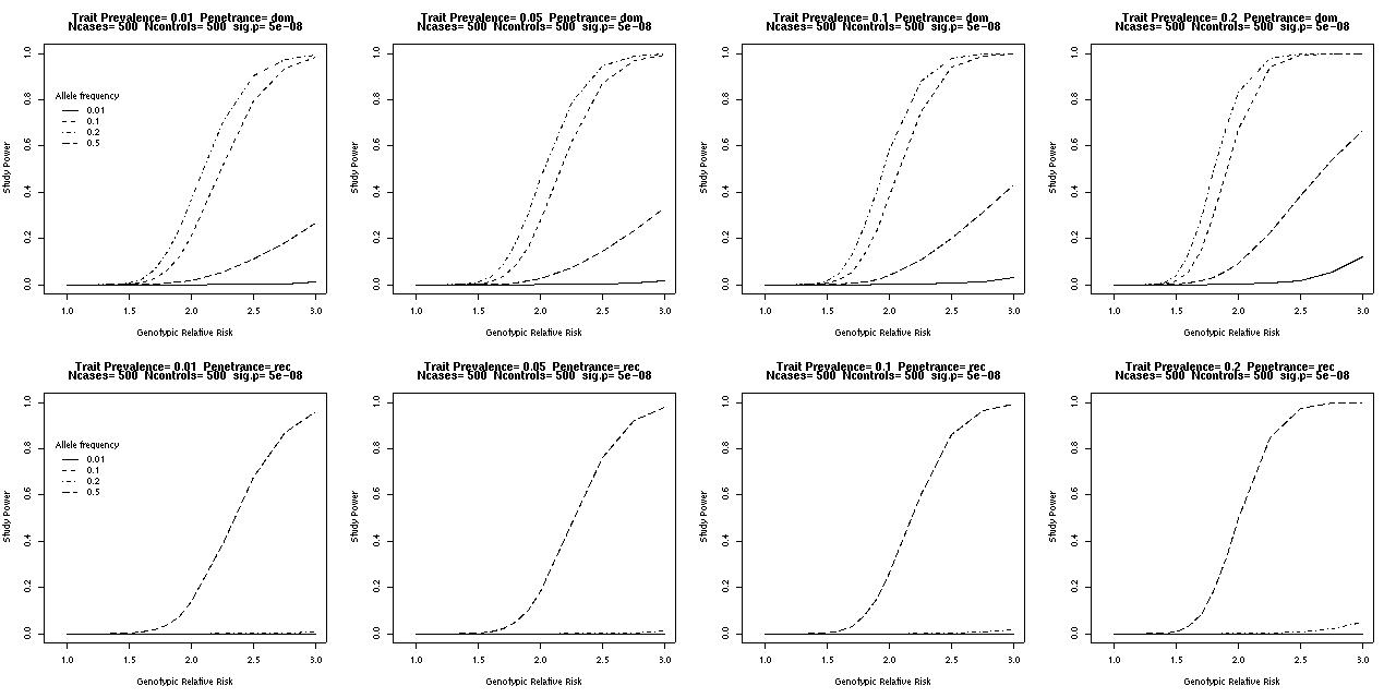
A moderately common dominant allele can be detected easily using a sample of this size, if there is the one locus acting, no confounding by environmental factors or stratification, and so forth.
| Genotype at D13S170 | ||||
|---|---|---|---|---|
| Fam | Father | Mother | Affected Child | Unaffected Child |
| 1 | 5/9 | 5/7 | 5/5 | 5/7 |
| 2 | 3/5 | 1/5 | 5/5 | 1/3 |
| 3a | 5/6 | 5/8 | 5/6 | 6/8 |
| 3b | 5/8 | 5/7 | 5/5 | 5/8 |
| 4 | 5/8 | 2/4 | 2/5 | 2/8 |
| 5 | 6/10 | 4/10 | 6/10 | 10/10 |
| 6 | 3/11 | 3/10 | 3/3 | 3/10 |
| 7 | 3/7 | 4/7 | 7/7 | 4/7 |
| 8 | -- | 2/5 | 5/5 | 2/5 (and 5/8) |
| 9 | 2/5 | 5/5 | 2/5 | 5/5 |
| 10 | 5/7 | 5/7 | 5/5 | 5/7 |
| 11 | 3/4 | 4/4 | 4/4 | 4/4 |
Is there evidence of association between D13S170 and LINCL? Are these loci linked? Allowing for the ascertainment, what is your best estimate of the marker allele frequencies in the general population (assume c=0)?